MEC3456 Lab 02: Implementation and Analysis of Interpolation Methods

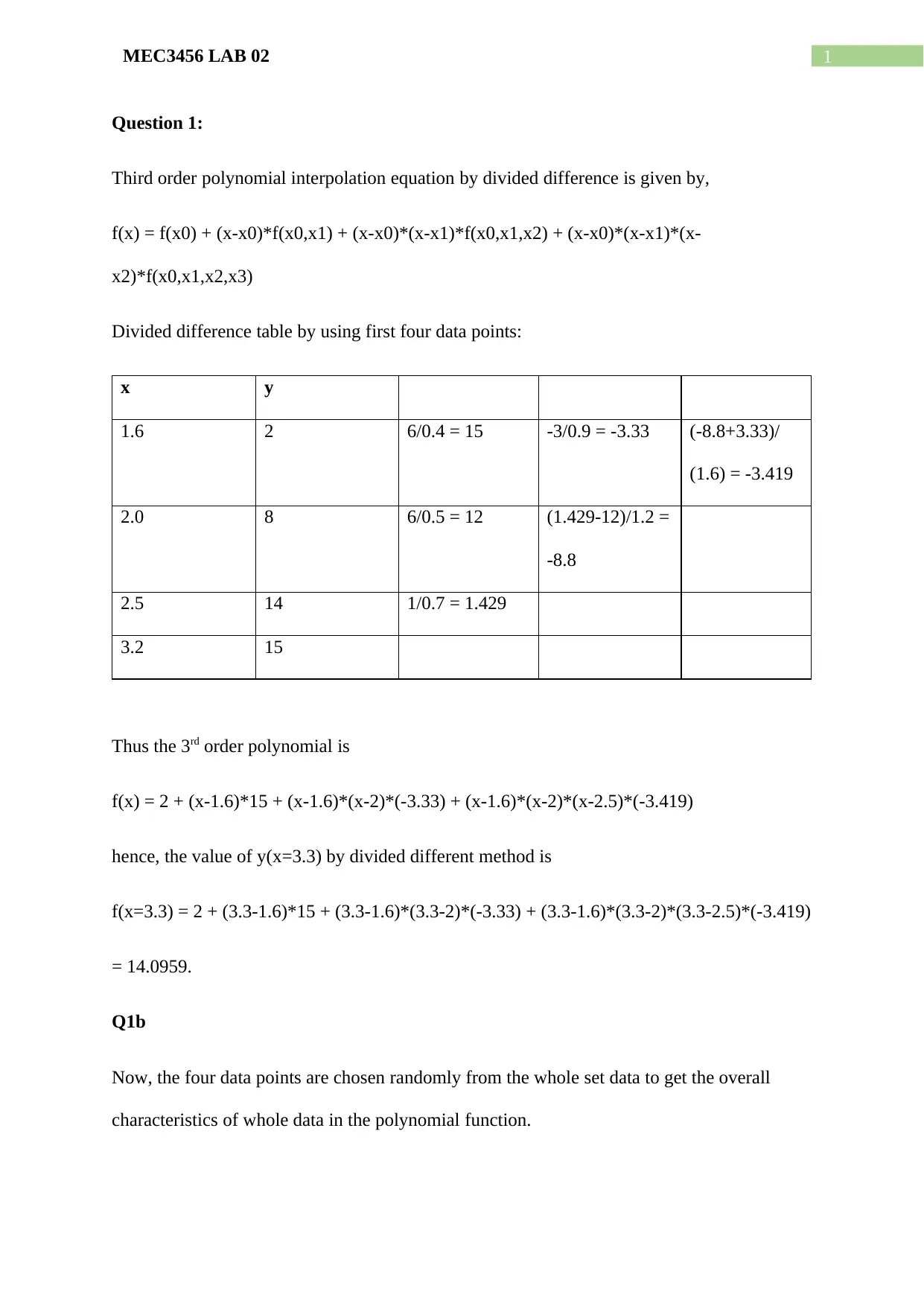
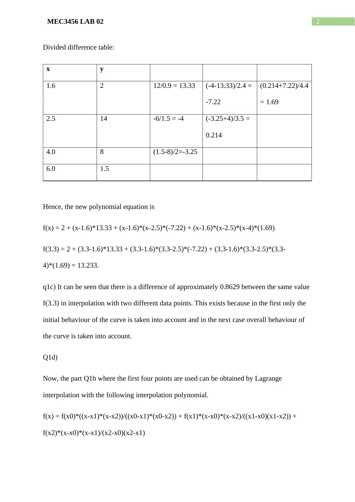
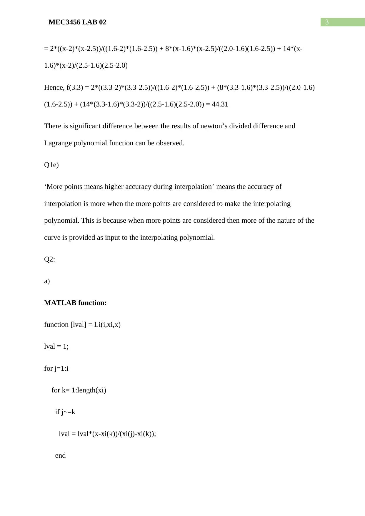
This document presents the solution to a Mechanical Engineering lab assignment (MEC3456 Lab 02) focusing on polynomial interpolation methods. The assignment explores divided difference and Lagrange interpolation techniques. The solution includes the derivation of a third-order polynomial interpolation equation using divided differences, demonstrating the calculation of y-values and analyzing the impact of data point selection on interpolation accuracy. It also involves the implementation of Lagrange interpolation using MATLAB, including functions for calculating Lagrange polynomials and interpolating data. The MATLAB code for both 1D and 2D interpolation, along with the analysis of the interpolation results and graphical representation of the data, is also provided. The assignment concludes with a discussion on the accuracy and limitations of different interpolation approaches.

Running head: MEC3456 LAB 02
MEC3456 LAB 02
Name of the Student
Name of the University
Author Note

1MEC3456 LAB 02
Question 1:
Third order polynomial interpolation equation by divided difference is given by,
f(x) = f(x0) + (x-x0)*f(x0,x1) + (x-x0)*(x-x1)*f(x0,x1,x2) + (x-x0)*(x-x1)*(x-
x2)*f(x0,x1,x2,x3)
Divided difference table by using first four data points:
x y
1.6 2 6/0.4 = 15 -3/0.9 = -3.33 (-8.8+3.33)/
(1.6) = -3.419
2.0 8 6/0.5 = 12 (1.429-12)/1.2 =
-8.8
2.5 14 1/0.7 = 1.429
3.2 15
Thus the 3rd order polynomial is
f(x) = 2 + (x-1.6)*15 + (x-1.6)*(x-2)*(-3.33) + (x-1.6)*(x-2)*(x-2.5)*(-3.419)
hence, the value of y(x=3.3) by divided different method is
f(x=3.3) = 2 + (3.3-1.6)*15 + (3.3-1.6)*(3.3-2)*(-3.33) + (3.3-1.6)*(3.3-2)*(3.3-2.5)*(-3.419)
= 14.0959.
Q1b
Now, the four data points are chosen randomly from the whole set data to get the overall
characteristics of whole data in the polynomial function.

2MEC3456 LAB 02
Divided difference table:
x y
1.6 2 12/0.9 = 13.33 (-4-13.33)/2.4 =
-7.22
(0.214+7.22)/4.4
= 1.69
2.5 14 -6/1.5 = -4 (-3.25+4)/3.5 =
0.214
4.0 8 (1.5-8)/2=-3.25
6.0 1.5
Hence, the new polynomial equation is
f(x) = 2 + (x-1.6)*13.33 + (x-1.6)*(x-2.5)*(-7.22) + (x-1.6)*(x-2.5)*(x-4)*(1.69)
f(3.3) = 2 + (3.3-1.6)*13.33 + (3.3-1.6)*(3.3-2.5)*(-7.22) + (3.3-1.6)*(3.3-2.5)*(3.3-
4)*(1.69) = 13.233.
q1c) It can be seen that there is a difference of approximately 0.8629 between the same value
f(3.3) in interpolation with two different data points. This exists because in the first only the
initial behaviour of the curve is taken into account and in the next case overall behaviour of
the curve is taken into account.
Q1d)
Now, the part Q1b where the first four points are used can be obtained by Lagrange
interpolation with the following interpolation polynomial.
f(x) = f(x0)*((x-x1)*(x-x2))/((x0-x1)*(x0-x2)) + f(x1)*(x-x0)*(x-x2)/((x1-x0)(x1-x2)) +
f(x2)*(x-x0)*(x-x1)/(x2-x0)(x2-x1)

3MEC3456 LAB 02
= 2*((x-2)*(x-2.5))/((1.6-2)*(1.6-2.5)) + 8*(x-1.6)*(x-2.5)/((2.0-1.6)(1.6-2.5)) + 14*(x-
1.6)*(x-2)/(2.5-1.6)(2.5-2.0)
Hence, f(3.3) = 2*((3.3-2)*(3.3-2.5))/((1.6-2)*(1.6-2.5)) + (8*(3.3-1.6)*(3.3-2.5))/((2.0-1.6)
(1.6-2.5)) + (14*(3.3-1.6)*(3.3-2))/((2.5-1.6)(2.5-2.0)) = 44.31
There is significant difference between the results of newton’s divided difference and
Lagrange polynomial function can be observed.
Q1e)
‘More points means higher accuracy during interpolation’ means the accuracy of
interpolation is more when the more points are considered to make the interpolating
polynomial. This is because when more points are considered then more of the nature of the
curve is provided as input to the interpolating polynomial.
Q2:
a)
MATLAB function:
function [lval] = Li(i,xi,x)
lval = 1;
for j=1:i
for k= 1:length(xi)
if j~=k
lval = lval*(x-xi(k))/(xi(j)-xi(k));
end

4MEC3456 LAB 02
end
end
end
Q2b:
MATLAB function:
function [yval] = LagrangeP(xi,yi,x)
yval = 0;
for j = 1:length(xi)
u = 1;
l = 1;
for k = 1:length(xi)
if j ~= k
u = u * (x - xi(j));
l = l * (xi(j) - xi(k));
end
end
yval= yval + u / l * yi(j);
end
end
Q2c:
MATLAB code:
% Q2c script file for Lab02
% Name
% Date
% Student ID
% Set up function f(x)
func = @(x) 1/(1+20*x^2);
% Set up 20 equidistant points and evaluate f(x)
x20 = linspace(-1,1,20);
for i=1:length(x20)
f20(i) = func(x20(i));
end
% Set up 100 points within [-1 1]
x100 = linspace(-1,1,100);
for i=1:length(x100)
f100(i) = func(x100(i));
end

5MEC3456 LAB 02
% Interpolate
for i=1:length(x100)
y100(i)= LagrangeP(x100,f100,x100(i));
end
% Plot and comment
plot(x20,f20,'r.',x100,y100,'b-')
title('Comparison of original points with Lagranges polynomial')
legend('20 data points','Interpolated polynomial with 100 data points')
xlabel('X values')
ylabel('Y values')
grid on
fprintf('The lagrange polynomial perfectly fits data points in middle
interval but end behaviour explaination is not good\n')
error = abs(y100-f100);
fprintf('The overall accuracy of interpolation is not good as the absolute
error is %.2f\n',error)
Output:
The lagrange polynomial perfectly fits data points in middle interval but end behaviour
explaination is not good
The overall accuracy of interpolation is not good as the absolute error is
615824319732054034476205106060591104.00

6MEC3456 LAB 02
-1 -0.8 -0.6 -0.4 -0.2 0 0.2 0.4 0.6 0.8 1
X values
-1
0
1
2
3
4
Y values
1037Comparison of original points with Lagranges polynomial
20 data points
Interpolated polynomial with 100 data points
Question 3:
a)
MATLAB function:
function [A] = LagrangeP_2D(m,n,xp,yp,fp,x,y)
xCurves={};
for i=1:m
% x vector must be a column vector for the lagrange function
x = xp';
% z vector must be a column vector for the lagrange function
z = fp(i,:)';
p=[];
for j = x(1:end)
% interpolate for every parameter value j and add it to p
p = [p,lagrange(x,z,j)];
end
% save curves in x direction
xCurves{i} = p;
end
y = yp;
% matrix for the graphical outpu
A=[];

7MEC3456 LAB 02
% interpolate in y-direction
for i=1:n
p=[];
z=[];
for l=1:length(y)
z = [z;xCurves{l}(i)];
end
for j = y(1:end)
% interpolate for every parameter value j and add it to p
p = [p;lagrange(y,z,j)];
end
A = [A,p];
end
end
b)
MATLAB code:
% Q3c script file for Lab02
% Name
% Date
% Student ID
% Define the data points
xmin = 0; % smallest value of x
xmax = 8; % largest value of x
xp = xmin:1:xmax;
yp = xp;
Np = length(xp);
% Define file to be read
fileID = fopen('temperature.dat','r');
% Define the format of the data to read and the shape of the output array.
Dformat = '%f %f';
sizeD = [Np Np];
% Read the file data into array, D (done in column order)
T = fscanf(fileID,Dformat,sizeD);
% Set up the grids needed.
[X,Y] = meshgrid(xp,yp);
Z = T;
step = 0.2;
xCurves={};
for i=1:size(X,1)
x = X(i,:)';

8MEC3456 LAB 02
z = Z(i,:)';
p=[];
for j = x(1):step:x(end)
p = [p,LagrangeP(x,z,j)];
end
xCurves{i} = p;
end
y = Y(:,1);
A=[];
for i=1:length(xCurves{1})
p=[];
z=[];
for l=1:length(y)
z = [z;xCurves{l}(i)];
end
for j = y(1):step:y(end)
p = [p;LagrangeP(y,z,j)];
end
A = [A,p];
end
% surface plot of the interpolated temperature
figure
surf(x(1):(x(end)-x(1))/(size(A,1)-1):x(end),y(1):(y(end)-y(1))/(size(A,1)-
1):y(end),A);
xlabel('x')
ylabel('y')
zlabel('temperature')
grid on
title('Plot of interpolated temperature')
figure
% plotting grid points
for i=1:size(X,1)
for j=1:size(Y,1)
p = plot3(X(i,j),Y(i,j),Z(i,j));
hold on
set(p,'Marker','.');
set(p,'MarkerSize',30);
end
end
title('Plot of grid points')
grid on
xlabel('x')
ylabel('y')
zlabel('temperature')
Output:

9MEC3456 LAB 02
-6
8
-4
-2
6 8
0
temperature
106
2
Plot of interpolated temperature
6
y
4
4
x
6
4
2 2
0 0
0
8
20
40
6 8
temperature
60
Plot of grid points
6
y
80
4
x
100
4
2 2
0 0

10MEC3456 LAB 02