Population Growth and Food Availability: Can Earth Feed 9 Billion?
VerifiedAdded on 2022/08/13
|26
|6110
|16
Report
AI Summary
This report investigates the critical question of whether the Earth can feed a projected population of 9 billion people, focusing on the interplay between population growth and food availability. It employs both exponential and logistic growth models to project future population sizes, comparing these projections with UN forecasts. The study analyzes the potential impact of these growth models on global food security, using wheat production data as a key indicator. The analysis includes the calculation of percentage changes in wheat production over several decades to project future food supply. The report assesses the challenges of feeding a growing population and suggests potential solutions, addressing issues of resource management and sustainable agricultural practices. The report concludes by emphasizing the need for a balance between agricultural production and population growth to mitigate the risks associated with food shortages and ensure a sustainable future.
1
Can the Earth feed 9 billion people? Predicting population growth and its impact
on food availability?
Name:
Institution:
Course number and name:
Instructor’s name:
3rd March 2020
Can the Earth feed 9 billion people? Predicting population growth and its impact
on food availability?
Name:
Institution:
Course number and name:
Instructor’s name:
3rd March 2020
Paraphrase This Document
Need a fresh take? Get an instant paraphrase of this document with our AI Paraphraser
2
Can the Earth feed 9 billion people? Predicting population growth and its impact
on food availability
1. Introduction
Usually, we have seen images in the media, especially children, suffering from
hunger and poverty. More than one billion of today’s seven billion people suffer from
hunger (UNICEF, 2015). Will it be enough food to feed the increasing global
population in the future? Feeding the world will be a huge challenge for humanity.
The issues of hunger and poverty are dealt in the framework of Sustainable
Development Goals and more specifically in SDG1 and SDG2. In this context,
concepts such as exponential growth, human carrying capacity and food availability
are extremely relevant in this context. Exponential growth "only occurs when a
species lives under optimal conditions, with enough food, water and space... and
above a certain population size, the growth rate slows down gradually" (Rutherford,
2009, p. 160-161). Population sizes are usually close to the carrying capacity, defined
as the maximum of human population that, the Earth can sustainably carry or support
(ibid.). This is a complex issue for a number of reasons. Among these reasons are that
humans use much more natural resources than any other animal. Also, the use of
resources varies according to differences in economic situation, culture and lifestyles.
Consequently, the question, how many people can the Earth support, cannot be easily
answered numerically. This means, that any estimates of human carrying capacity
depend on the choices we are going to make in the future as well as natural events.
We have also to keep in mind that population is increasing at a higher rate than
agricultural production (FAO, 2007) as well as that a lot of food is wasted. Reaching a
balance between the agricultural production and the rate of population growth can
limit the risks associated with a lack of food.
3
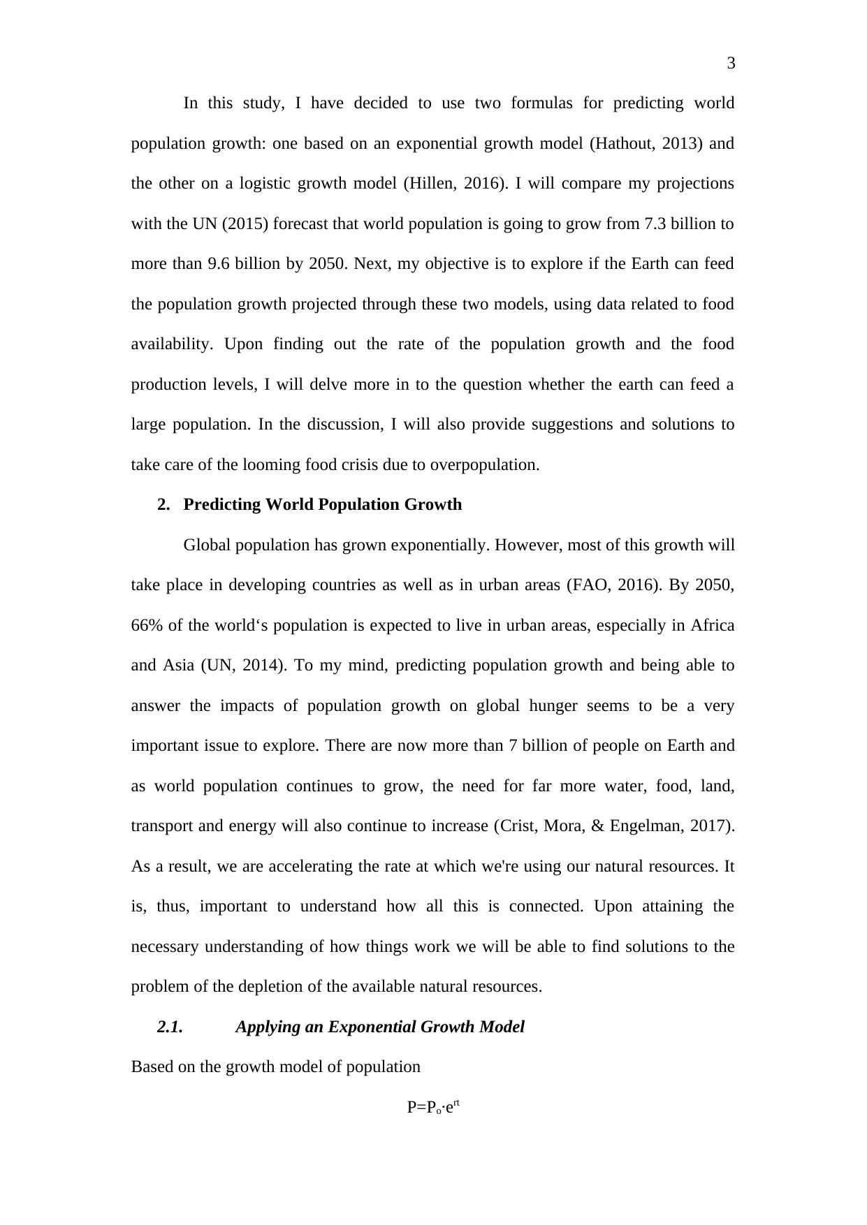
In this study, I have decided to use two formulas for predicting world
population growth: one based on an exponential growth model (Hathout, 2013) and
the other on a logistic growth model (Hillen, 2016). I will compare my projections
with the UN (2015) forecast that world population is going to grow from 7.3 billion to
more than 9.6 billion by 2050. Next, my objective is to explore if the Earth can feed
the population growth projected through these two models, using data related to food
availability. Upon finding out the rate of the population growth and the food
production levels, I will delve more in to the question whether the earth can feed a
large population. In the discussion, I will also provide suggestions and solutions to
take care of the looming food crisis due to overpopulation.
2. Predicting World Population Growth
Global population has grown exponentially. However, most of this growth will
take place in developing countries as well as in urban areas (FAO, 2016). By 2050,
66% of the world‘s population is expected to live in urban areas, especially in Africa
and Asia (UN, 2014). To my mind, predicting population growth and being able to
answer the impacts of population growth on global hunger seems to be a very
important issue to explore. There are now more than 7 billion of people on Earth and
as world population continues to grow, the need for far more water, food, land,
transport and energy will also continue to increase (Crist, Mora, & Engelman, 2017).
As a result, we are accelerating the rate at which we're using our natural resources. It
is, thus, important to understand how all this is connected. Upon attaining the
necessary understanding of how things work we will be able to find solutions to the
problem of the depletion of the available natural resources.
2.1. Applying an Exponential Growth Model
Based on the growth model of population
P=Po∙ert
⊘ This is a preview!⊘
Do you want full access?
Subscribe today to unlock all pages.
Trusted by 1+ million students worldwide
4
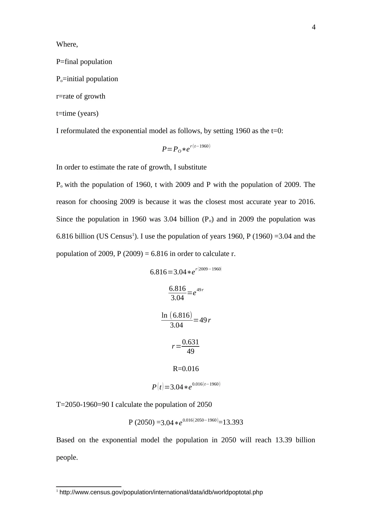
Where,
P=final population
Po=initial population
r=rate of growth
t=time (years)
I reformulated the exponential model as follows, by setting 1960 as the t=0:
P=PO∗er (t−1960)
In order to estimate the rate of growth, I substitute
Po with the population of 1960, t with 2009 and P with the population of 2009. The
reason for choosing 2009 is because it was the closest most accurate year to 2016.
Since the population in 1960 was 3.04 billion (Po) and in 2009 the population was
6.816 billion (US Census1). I use the population of years 1960, P (1960) =3.04 and the
population of 2009, P (2009) = 6.816 in order to calculate r.
6.816=3.04∗er ( 2009−1960)
6.816
3.04 =e49 r
ln (6.816)
3.04 =49 r
r =0.631
49
R=0.016
P ( t ) =3.04∗e0.016(t−1960)
T=2050-1960=90 I calculate the population of 2050
P (2050) =3.04∗e0.016(2050−1960)=13.393
Based on the exponential model the population in 2050 will reach 13.39 billion
people.
1 http://www.census.gov/population/international/data/idb/worldpoptotal.php
Paraphrase This Document
Need a fresh take? Get an instant paraphrase of this document with our AI Paraphraser
5
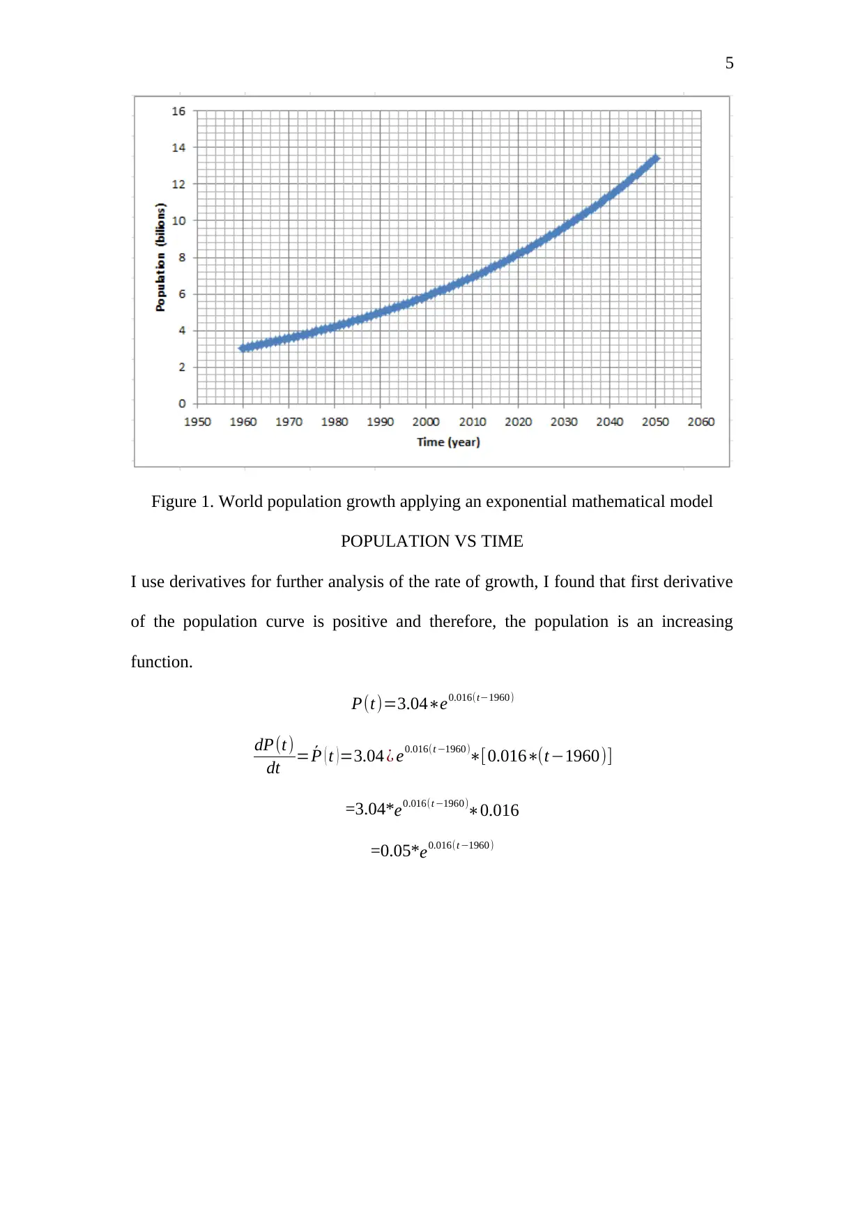
Figure 1. World population growth applying an exponential mathematical model
POPULATION VS TIME
I use derivatives for further analysis of the rate of growth, I found that first derivative
of the population curve is positive and therefore, the population is an increasing
function.
P(t)=3.04∗e0.016(t−1960)
dP(t)
dt = ´P ( t )=3.04 ¿ e0.016(t −1960)∗[0.016∗(t−1960)]
=3.04*e0.016(t −1960)∗0.016
=0.05*e0.016(t −1960)
6
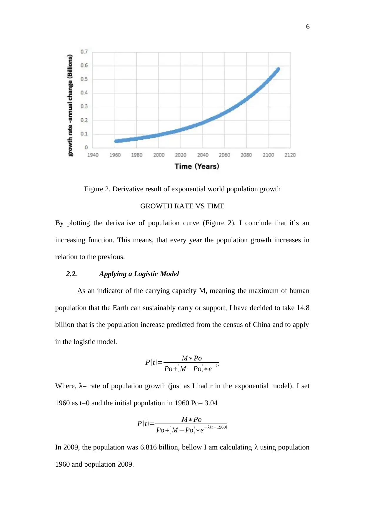
Figure 2. Derivative result of exponential world population growth
GROWTH RATE VS TIME
By plotting the derivative of population curve (Figure 2), I conclude that it’s an
increasing function. This means, that every year the population growth increases in
relation to the previous.
2.2. Applying a Logistic Model
As an indicator of the carrying capacity M, meaning the maximum of human
population that the Earth can sustainably carry or support, I have decided to take 14.8
billion that is the population increase predicted from the census of China and to apply
in the logistic model.
P ( t ) = M∗Po
Po+ ( M −Po ) ∗e− λt
Where, λ= rate of population growth (just as I had r in the exponential model). I set
1960 as t=0 and the initial population in 1960 Po= 3.04
P ( t ) = M∗Po
Po+ ( M −Po ) ∗e− λ(t −1960)
In 2009, the population was 6.816 billion, bellow I am calculating λ using population
1960 and population 2009.
⊘ This is a preview!⊘
Do you want full access?
Subscribe today to unlock all pages.
Trusted by 1+ million students worldwide
7
6.816= 44.995
3.04 +11.76∗e−49 λ
3.04+11.76∗e−49 λ= 6.602
11.76∗e−49 λ= 6.602-3.04
e−49 λ= 6.602−3.04
11.76
e−49 λ=0.303
lne−49 λ=ln 0.303
−49 λ=−1.195
λ=−1.195
−49
λ=0.024
P(t)= 44.326
3.04 +11.759∗e−0.024(t−1960)
P(2050)= 44.326
3.04+11.759∗e−0.024 (2050 −1960)
P ( t ) = 44.326
3.04 +11.759∗e−0.024∗90 =10.18
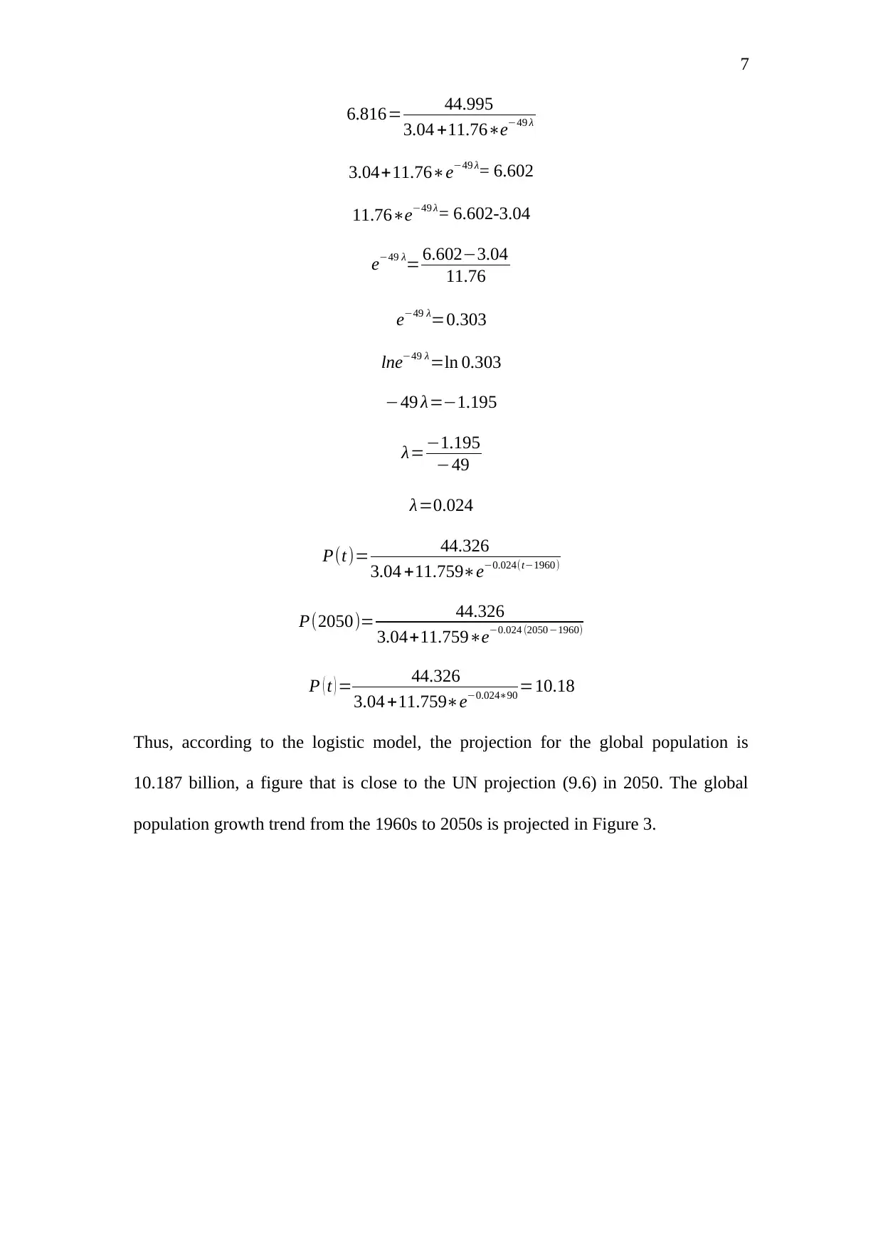
Thus, according to the logistic model, the projection for the global population is
10.187 billion, a figure that is close to the UN projection (9.6) in 2050. The global
population growth trend from the 1960s to 2050s is projected in Figure 3.
6.816= 44.995
3.04 +11.76∗e−49 λ
3.04+11.76∗e−49 λ= 6.602
11.76∗e−49 λ= 6.602-3.04
e−49 λ= 6.602−3.04
11.76
e−49 λ=0.303
lne−49 λ=ln 0.303
−49 λ=−1.195
λ=−1.195
−49
λ=0.024
P(t)= 44.326
3.04 +11.759∗e−0.024(t−1960)
P(2050)= 44.326
3.04+11.759∗e−0.024 (2050 −1960)
P ( t ) = 44.326
3.04 +11.759∗e−0.024∗90 =10.18
Thus, according to the logistic model, the projection for the global population is
10.187 billion, a figure that is close to the UN projection (9.6) in 2050. The global
population growth trend from the 1960s to 2050s is projected in Figure 3.
Paraphrase This Document
Need a fresh take? Get an instant paraphrase of this document with our AI Paraphraser
8
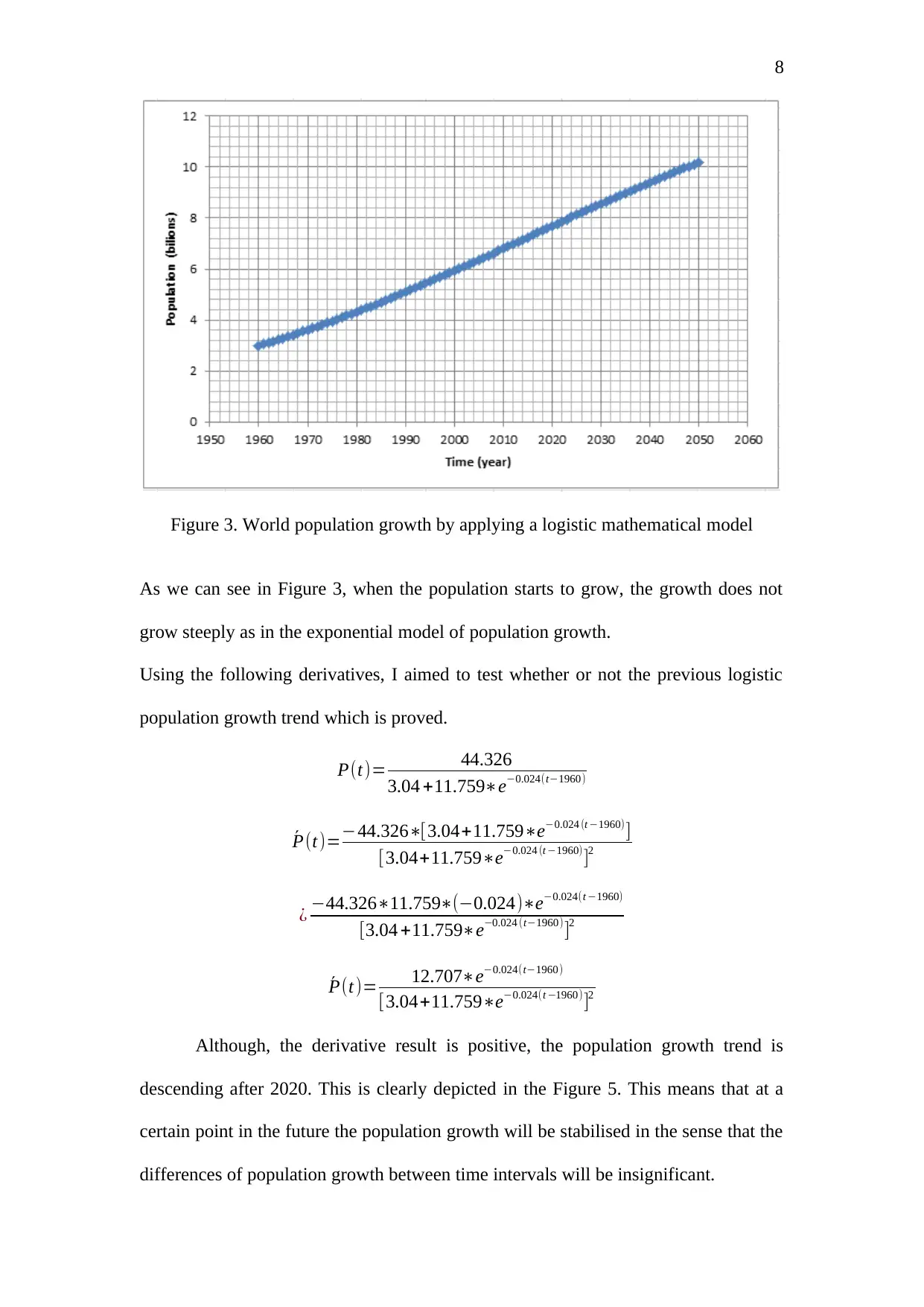
Figure 3. World population growth by applying a logistic mathematical model
As we can see in Figure 3, when the population starts to grow, the growth does not
grow steeply as in the exponential model of population growth.
Using the following derivatives, I aimed to test whether or not the previous logistic
population growth trend which is proved.
P(t)= 44.326
3.04 +11.759∗e−0.024(t−1960)
´P(t)=−44.326∗[3.04+11.759∗e−0.024 (t −1960)]
[3.04+11.759∗e−0.024 (t −1960)]2
¿ −44.326∗11.759∗(−0.024)∗e−0.024(t −1960)
[3.04 +11.759∗e−0.024 (t−1960)]2
´P(t)= 12.707∗e−0.024(t−1960)
[3.04+11.759∗e−0.024(t −1960)]2
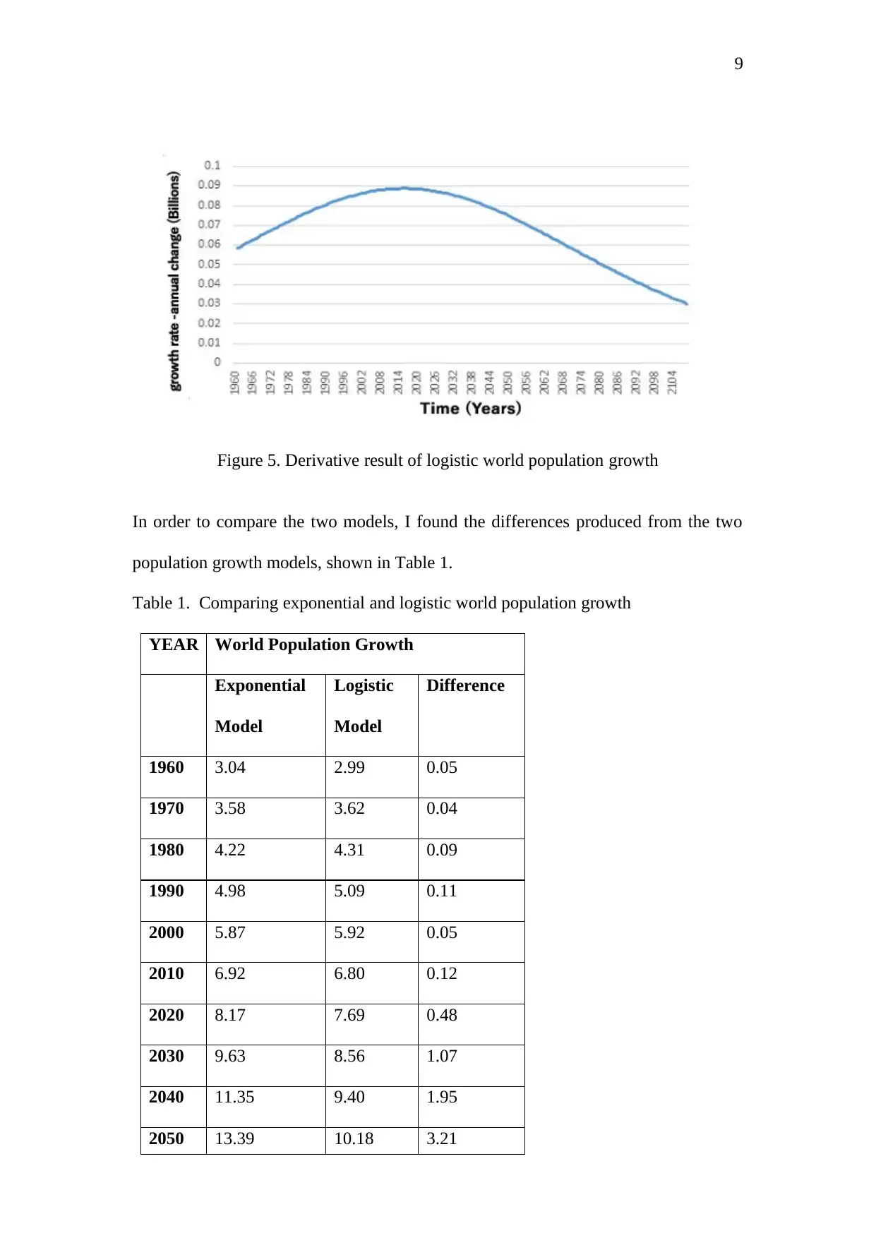
Although, the derivative result is positive, the population growth trend is
descending after 2020. This is clearly depicted in the Figure 5. This means that at a
certain point in the future the population growth will be stabilised in the sense that the
differences of population growth between time intervals will be insignificant.
Figure 3. World population growth by applying a logistic mathematical model
As we can see in Figure 3, when the population starts to grow, the growth does not
grow steeply as in the exponential model of population growth.
Using the following derivatives, I aimed to test whether or not the previous logistic
population growth trend which is proved.
P(t)= 44.326
3.04 +11.759∗e−0.024(t−1960)
´P(t)=−44.326∗[3.04+11.759∗e−0.024 (t −1960)]
[3.04+11.759∗e−0.024 (t −1960)]2
¿ −44.326∗11.759∗(−0.024)∗e−0.024(t −1960)
[3.04 +11.759∗e−0.024 (t−1960)]2
´P(t)= 12.707∗e−0.024(t−1960)
[3.04+11.759∗e−0.024(t −1960)]2
Although, the derivative result is positive, the population growth trend is
descending after 2020. This is clearly depicted in the Figure 5. This means that at a
certain point in the future the population growth will be stabilised in the sense that the
differences of population growth between time intervals will be insignificant.
9
Figure 5. Derivative result of logistic world population growth
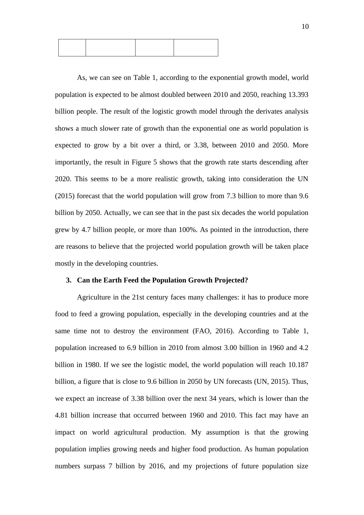
In order to compare the two models, I found the differences produced from the two
population growth models, shown in Table 1.
Table 1. Comparing exponential and logistic world population growth
YEAR World Population Growth
Exponential
Model
Logistic
Model
Difference
1960 3.04 2.99 0.05
1970 3.58 3.62 0.04
1980 4.22 4.31 0.09
1990 4.98 5.09 0.11
2000 5.87 5.92 0.05
2010 6.92 6.80 0.12
2020 8.17 7.69 0.48
2030 9.63 8.56 1.07
2040 11.35 9.40 1.95
2050 13.39 10.18 3.21
Figure 5. Derivative result of logistic world population growth
In order to compare the two models, I found the differences produced from the two
population growth models, shown in Table 1.
Table 1. Comparing exponential and logistic world population growth
YEAR World Population Growth
Exponential
Model
Logistic
Model
Difference
1960 3.04 2.99 0.05
1970 3.58 3.62 0.04
1980 4.22 4.31 0.09
1990 4.98 5.09 0.11
2000 5.87 5.92 0.05
2010 6.92 6.80 0.12
2020 8.17 7.69 0.48
2030 9.63 8.56 1.07
2040 11.35 9.40 1.95
2050 13.39 10.18 3.21
⊘ This is a preview!⊘
Do you want full access?
Subscribe today to unlock all pages.
Trusted by 1+ million students worldwide
10
Αs, we can see on Table 1, according to the exponential growth model, world
population is expected to be almost doubled between 2010 and 2050, reaching 13.393
billion people. The result of the logistic growth model through the derivates analysis
shows a much slower rate of growth than the exponential one as world population is
expected to grow by a bit over a third, or 3.38, between 2010 and 2050. More
importantly, the result in Figure 5 shows that the growth rate starts descending after
2020. This seems to be a more realistic growth, taking into consideration the UN
(2015) forecast that the world population will grow from 7.3 billion to more than 9.6
billion by 2050. Actually, we can see that in the past six decades the world population
grew by 4.7 billion people, or more than 100%. As pointed in the introduction, there
are reasons to believe that the projected world population growth will be taken place
mostly in the developing countries.
3. Can the Earth Feed the Population Growth Projected?
Agriculture in the 21st century faces many challenges: it has to produce more
food to feed a growing population, especially in the developing countries and at the
same time not to destroy the environment (FAO, 2016). According to Table 1,
population increased to 6.9 billion in 2010 from almost 3.00 billion in 1960 and 4.2
billion in 1980. If we see the logistic model, the world population will reach 10.187
billion, a figure that is close to 9.6 billion in 2050 by UN forecasts (UN, 2015). Thus,
we expect an increase of 3.38 billion over the next 34 years, which is lower than the
4.81 billion increase that occurred between 1960 and 2010. This fact may have an
impact on world agricultural production. My assumption is that the growing
population implies growing needs and higher food production. As human population
numbers surpass 7 billion by 2016, and my projections of future population size
Paraphrase This Document
Need a fresh take? Get an instant paraphrase of this document with our AI Paraphraser
11
exceeds 13 billion in 2050 by applying the exponential growth model and 10 billion
by applying the logistic population growth model, the need to understand its impact
on feeding the human population becomes very pressing.
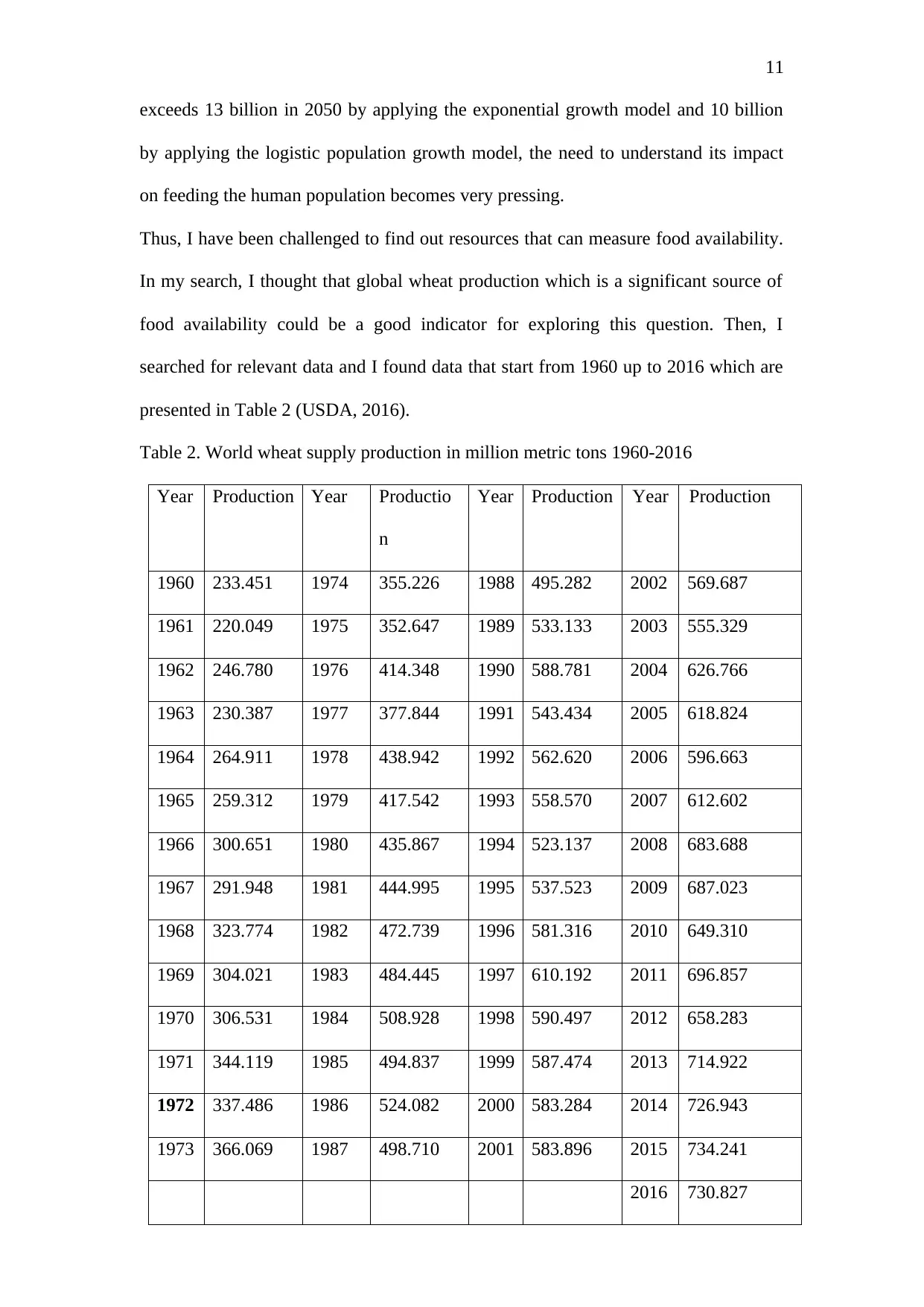
Thus, I have been challenged to find out resources that can measure food availability.
In my search, I thought that global wheat production which is a significant source of
food availability could be a good indicator for exploring this question. Then, I
searched for relevant data and I found data that start from 1960 up to 2016 which are
presented in Table 2 (USDA, 2016).
Table 2. World wheat supply production in million metric tons 1960-2016
Year Production Year Productio
n
Year Production Year Production
1960 233.451 1974 355.226 1988 495.282 2002 569.687
1961 220.049 1975 352.647 1989 533.133 2003 555.329
1962 246.780 1976 414.348 1990 588.781 2004 626.766
1963 230.387 1977 377.844 1991 543.434 2005 618.824
1964 264.911 1978 438.942 1992 562.620 2006 596.663
1965 259.312 1979 417.542 1993 558.570 2007 612.602
1966 300.651 1980 435.867 1994 523.137 2008 683.688
1967 291.948 1981 444.995 1995 537.523 2009 687.023
1968 323.774 1982 472.739 1996 581.316 2010 649.310
1969 304.021 1983 484.445 1997 610.192 2011 696.857
1970 306.531 1984 508.928 1998 590.497 2012 658.283
1971 344.119 1985 494.837 1999 587.474 2013 714.922
1972 337.486 1986 524.082 2000 583.284 2014 726.943
1973 366.069 1987 498.710 2001 583.896 2015 734.241
2016 730.827
exceeds 13 billion in 2050 by applying the exponential growth model and 10 billion
by applying the logistic population growth model, the need to understand its impact
on feeding the human population becomes very pressing.
Thus, I have been challenged to find out resources that can measure food availability.
In my search, I thought that global wheat production which is a significant source of
food availability could be a good indicator for exploring this question. Then, I
searched for relevant data and I found data that start from 1960 up to 2016 which are
presented in Table 2 (USDA, 2016).
Table 2. World wheat supply production in million metric tons 1960-2016
Year Production Year Productio
n
Year Production Year Production
1960 233.451 1974 355.226 1988 495.282 2002 569.687
1961 220.049 1975 352.647 1989 533.133 2003 555.329
1962 246.780 1976 414.348 1990 588.781 2004 626.766
1963 230.387 1977 377.844 1991 543.434 2005 618.824
1964 264.911 1978 438.942 1992 562.620 2006 596.663
1965 259.312 1979 417.542 1993 558.570 2007 612.602
1966 300.651 1980 435.867 1994 523.137 2008 683.688
1967 291.948 1981 444.995 1995 537.523 2009 687.023
1968 323.774 1982 472.739 1996 581.316 2010 649.310
1969 304.021 1983 484.445 1997 610.192 2011 696.857
1970 306.531 1984 508.928 1998 590.497 2012 658.283
1971 344.119 1985 494.837 1999 587.474 2013 714.922
1972 337.486 1986 524.082 2000 583.284 2014 726.943
1973 366.069 1987 498.710 2001 583.896 2015 734.241
2016 730.827
12
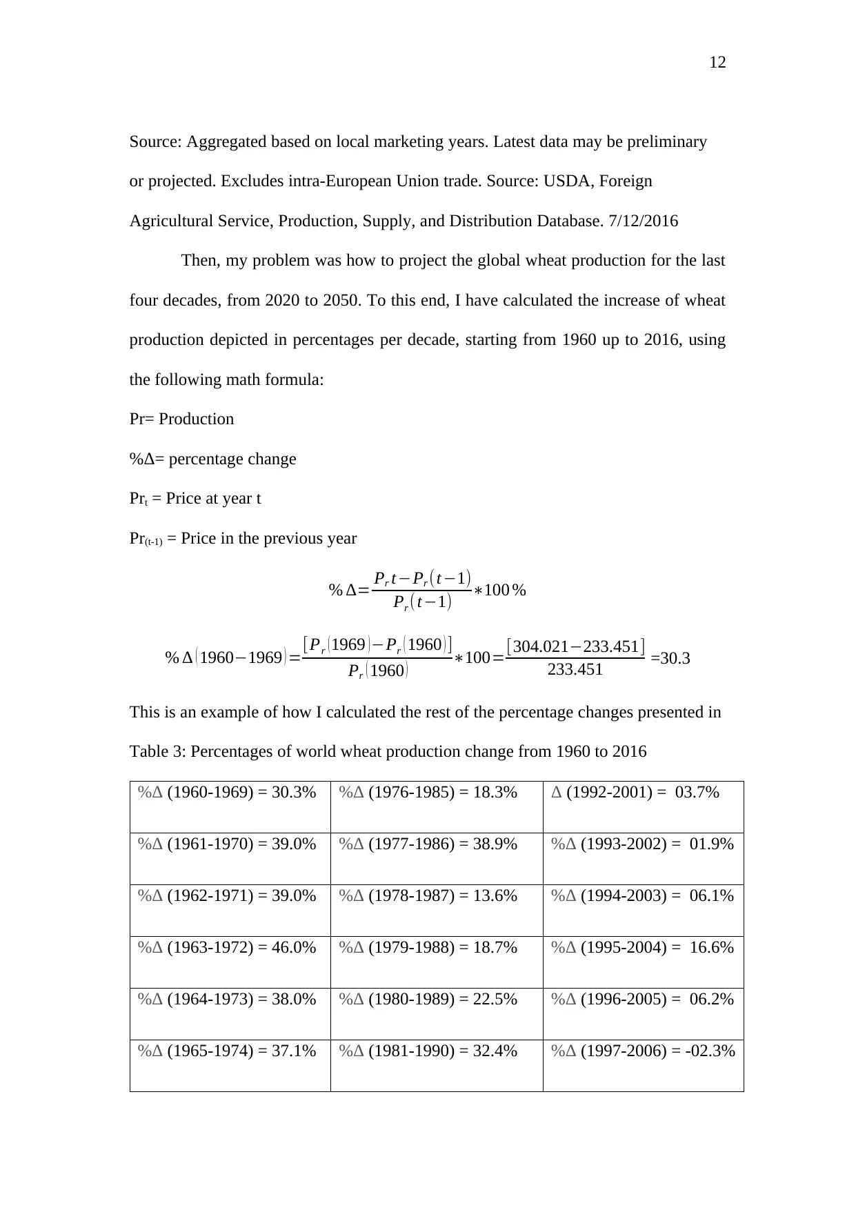
Source: Aggregated based on local marketing years. Latest data may be preliminary
or projected. Excludes intra-European Union trade. Source: USDA, Foreign
Agricultural Service, Production, Supply, and Distribution Database. 7/12/2016
Then, my problem was how to project the global wheat production for the last
four decades, from 2020 to 2050. To this end, I have calculated the increase of wheat
production depicted in percentages per decade, starting from 1960 up to 2016, using
the following math formula:
Pr= Production
%Δ= percentage change
Prt = Price at year t
Pr(t-1) = Price in the previous year
% ∆= Pr t−Pr (t−1)
Pr (t−1) ∗100 %
% ∆ ( 1960−1969 ) =[Pr (1969 )−Pr ( 1960 ) ]
Pr ( 1960 ) ∗100=[304.021−233.451]
233.451 =30.3
This is an example of how I calculated the rest of the percentage changes presented in
Table 3: Percentages of world wheat production change from 1960 to 2016
%Δ (1960-1969) = 30.3% %Δ (1976-1985) = 18.3% Δ (1992-2001) = 03.7%
%Δ (1961-1970) = 39.0% %Δ (1977-1986) = 38.9% %Δ (1993-2002) = 01.9%
%Δ (1962-1971) = 39.0% %Δ (1978-1987) = 13.6% %Δ (1994-2003) = 06.1%
%Δ (1963-1972) = 46.0% %Δ (1979-1988) = 18.7% %Δ (1995-2004) = 16.6%
%Δ (1964-1973) = 38.0% %Δ (1980-1989) = 22.5% %Δ (1996-2005) = 06.2%
%Δ (1965-1974) = 37.1% %Δ (1981-1990) = 32.4% %Δ (1997-2006) = -02.3%
⊘ This is a preview!⊘
Do you want full access?
Subscribe today to unlock all pages.
Trusted by 1+ million students worldwide
1 out of 26
Related Documents


Your All-in-One AI-Powered Toolkit for Academic Success.
+13062052269
info@desklib.com
Available 24*7 on WhatsApp / Email
![[object Object]](/_next/static/media/star-bottom.7253800d.svg)
Unlock your academic potential
Copyright © 2020–2026 A2Z Services. All Rights Reserved. Developed and managed by ZUCOL.