Data Analysis: Health and Population Statistics of East Asia

This report presents a data analysis of health and population statistics in the East Asia and Pacific region from 2001 to 2015, utilizing data from the World Bank. The analysis investigates the relationship between crude birth and death rates, health expenditure, and population growth. The methodology includes exploratory data analysis with one and two variable analyses using box plots and histograms, followed by advanced techniques such as k-means clustering to group countries with similar birth and death rates, and linear regression to identify relationships between variables. The report explores the distribution of crude death and birth rates, and the impact of health expenditure on population growth and immunization rates. The findings are crucial for governments and planners in resource allocation to improve health outcomes. The study is limited to the East Asia and Pacific region. The report concludes with key insights derived from the statistical analyses and visualizations.

Data analysis report of the health and population statistics of East Asian and Pacific countries
Name of the Student

Table of Contents
1 Introduction..................................................................................................................................1
1.1 Authorisation and Purpose....................................................................................................1
Limitations...................................................................................................................................1
Scope............................................................................................................................................1
Methodology...............................................................................................................................1
2 Data Setup....................................................................................................................................1
3 Exploratory Data Analysis.............................................................................................................2
3.1 One Variable Analysis................................................................................................................2
3.1.1 One Variable Analysis – 1.......................................................................................................2
3.1.2 One Variable Analysis – 2.......................................................................................................3
3.1.3 One Variable Analysis – 3.......................................................................................................5
3.2 Two-variable analysis.................................................................................................................6
3.2.1 Two-variable analysis 1...........................................................................................................6
3.2.2 Two-variable analysis 2...........................................................................................................7
4 Advanced analysis.........................................................................................................................8
4.1 Clustering...................................................................................................................................8
4.1.1 Brief explanation of k-means and clustering..........................................................................8
4.1.2 Clustering Analysis..................................................................................................................9
4.2 Linear regression......................................................................................................................10
4.2.1 Brief definition of linear regression......................................................................................10
4.2.2 Linear Regression 1...............................................................................................................10
4.2.3 Linear Regression 2...............................................................................................................12
5 Conclusion...................................................................................................................................13
6 Reflection....................................................................................................................................14
Reference.......................................................................................................................................15
Page | ii

1 Introduction
1.1 Authorisation and Purpose
Herein we investigate the health development of East Asia and Pacific Region during the period
of 2001 to 2015. The data for the investigation has been taken from world bank. The research
team is particularly interested in the relation of crude birth and death rate to the health
expenditure of the region. Moreover, in this research we intend to study how crude birth and
deaths rate have varied across countries for last 15 years. In addition, the research intends to
study the relation between growth in population of the region (the difference between crude
death rate and crude birth rate) and health expenditure. Further, the relation between
immunization rate and crude birth rate is studied.
The outcomes of the analysis have importance to government and planners. The analysis can be
utilised for resource mobilisation to improve the health of the country.
Limitations
The analysis is limited to the region of East Asia and Pacific only.
Scope
For analysing the health of the region the present study is segregated into four groups. Initially
the researcher evaluates the attributes using a one variable study. Box-plots and histograms are
used to undertake a one-attribute study. In the second part two of variables are studies. in
order to undertake the two variable study box-plots were found to be best suited. In the next
section the researcher has evaluated patterns in the relation between crude birth and death
rate. The countries of the region having similar death and birth rates have been grouped
together. Finally, in the last section, growth in population of the region is related to health
expenditure and birth rate to immunization rate.
Methodology
Quantitative data got from world bank is used for the present analysis. The data pertains to the
time period of 2001 to 2015 and East Asia and Pacific Region.
2 Data Setup
In order to undertake the analysis, the data file should be loaded into the R program. Thus the
first line of the code requests the user to load the required data file. During the process of
running the first line of code a window pops up and the data file to be analysed is requested.
The pre-processing of the data file also takes place when the data file is loaded. All missing
values are tagged and the first row is taken as the header row. In the second stage the required
library files are loaded. In order to undertake the analysis certain library files are required. The
library files are loaded in the second stage.

3 Exploratory Data Analysis
3.1 One Variable Analysis
3.1.1 One Variable Analysis – 1
The crude death rate of the region per 1000 people in 2014 is studied as a one-variable analysis.
In 2014 the average death rate was 6.37 with a standard deviation of 1.44 for every 1000
people. The minimum and maximum death rate was 2.99 and 10 respectively in the region. The
median death rate in 2014 was 6.16 for every 1000 people. From the analysis it can be seen
that the minimum and maximum death rates of the region are outliers.
Page | 2
fill <- "#4271AE"
line <- "#1F3552"
Analysis11 <- ggplot(Data1, aes(x = factor(0), y = SP.DYN.CDRT.IN)) + geom_boxplot(fill =
fill, colour = line, alpha = 0.7)
Analysis11 <- Analysis11 + scale_x_discrete(name = "Crude Death Rate (per 1000 people)")
+ scale_y_continuous(name = "Count")
Analysis11 <- Analysis11 + ggtitle("Distribution of Crude death Rate in the Region in 2014")
+ theme_bw()
describe(Data1$SP.DYN.CDRT.IN)
Analysis11
Data <- read.csv(file.choose(), header = TRUE, sep = "," , na.strings = "..")
# Loading required library files
library(data.table)
library(reshape2)
library(psych)
library(factoextra)
library(ggplot2)
library(lattice)
library(dplyr)

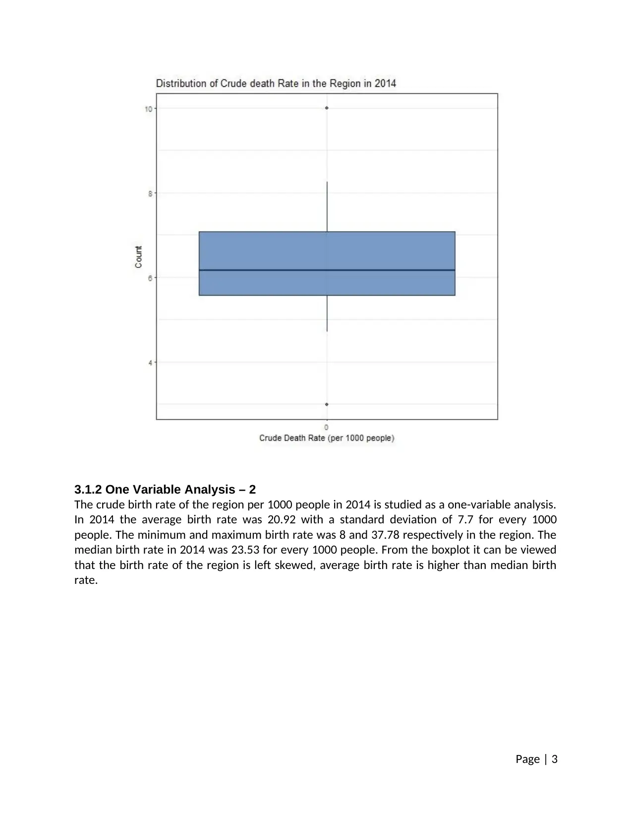
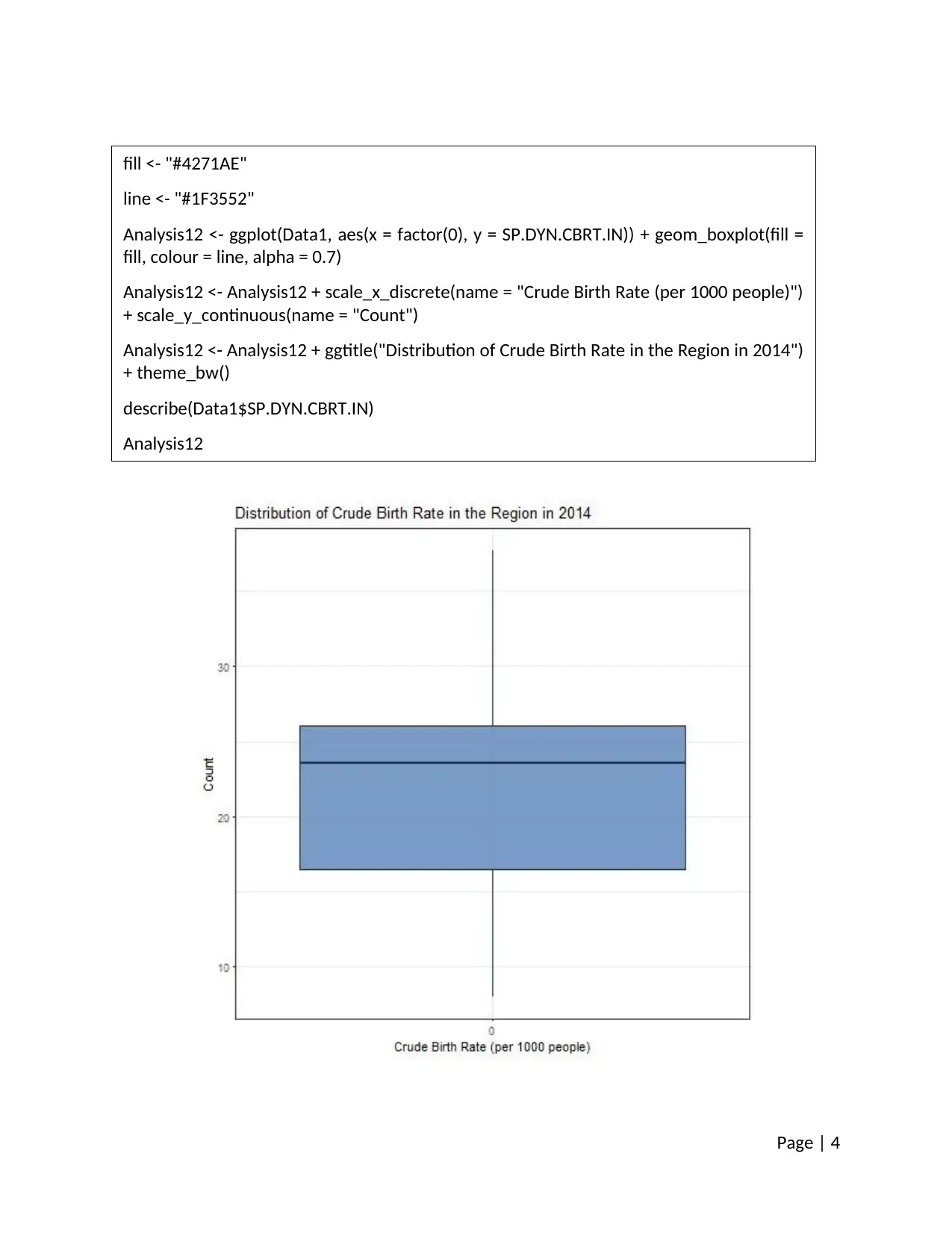
3.1.2 One Variable Analysis – 2
The crude birth rate of the region per 1000 people in 2014 is studied as a one-variable analysis.
In 2014 the average birth rate was 20.92 with a standard deviation of 7.7 for every 1000
people. The minimum and maximum birth rate was 8 and 37.78 respectively in the region. The
median birth rate in 2014 was 23.53 for every 1000 people. From the boxplot it can be viewed
that the birth rate of the region is left skewed, average birth rate is higher than median birth
rate.
Page | 3

Page | 4
fill <- "#4271AE"
line <- "#1F3552"
Analysis12 <- ggplot(Data1, aes(x = factor(0), y = SP.DYN.CBRT.IN)) + geom_boxplot(fill =
fill, colour = line, alpha = 0.7)
Analysis12 <- Analysis12 + scale_x_discrete(name = "Crude Birth Rate (per 1000 people)")
+ scale_y_continuous(name = "Count")
Analysis12 <- Analysis12 + ggtitle("Distribution of Crude Birth Rate in the Region in 2014")
+ theme_bw()
describe(Data1$SP.DYN.CBRT.IN)
Analysis12

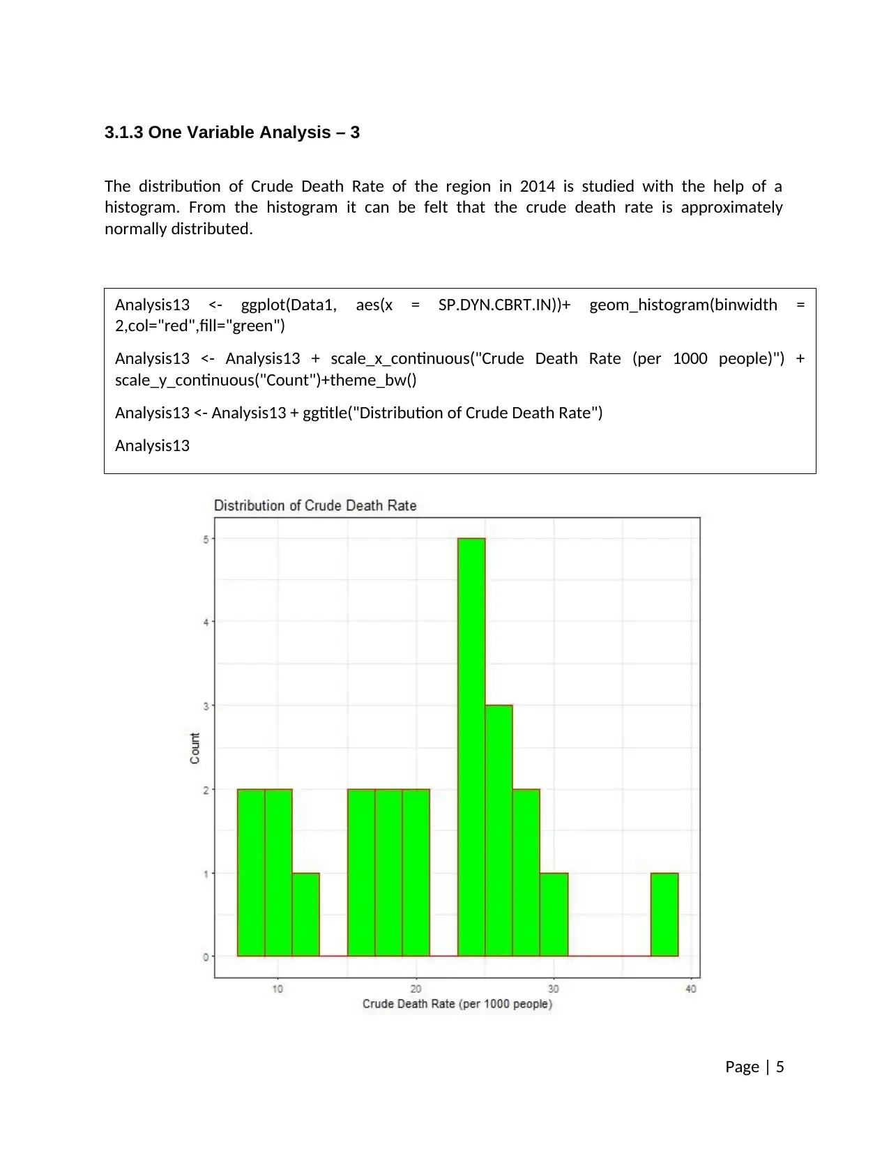
3.1.3 One Variable Analysis – 3
The distribution of Crude Death Rate of the region in 2014 is studied with the help of a
histogram. From the histogram it can be felt that the crude death rate is approximately
normally distributed.
Page | 5
Analysis13 <- ggplot(Data1, aes(x = SP.DYN.CBRT.IN))+ geom_histogram(binwidth =
2,col="red",fill="green")
Analysis13 <- Analysis13 + scale_x_continuous("Crude Death Rate (per 1000 people)") +
scale_y_continuous("Count")+theme_bw()
Analysis13 <- Analysis13 + ggtitle("Distribution of Crude Death Rate")
Analysis13

3.2 Two-variable analysis
3.2.1 Two-variable analysis 1
The spread of crude death rate of the region from 2001 to 2015 was studied in the two-variable
analysis. A boxplot with the names of the countries in the x-axis and the values in the y-axis is
plotted. The box-plots shows that the crude death rate of BRN (Brunei Darussalam) during the
period of study is the least. Further, there are wide variations in crude death rate of different
countries. Moreover, the crude death rate is skewed for most of the countries during the
period.
Page | 6
Data2a <- Data2[Series.Code %in% "SP.DYN.CDRT.IN"]
fill = "Orange"
Analysis21 <- ggplot(Data2a, aes(x = Data2a$Country.Code, y = Data2a$value)) +
geom_boxplot(fill = fill)
Analysis21 <- Analysis21 + scale_x_discrete(name = "Country") + scale_y_continuous(name =
"Crude Death Rate (per 1000 people)")+ theme_bw()
Analysis21 <- Analysis21 +theme(axis.text.x = element_text(angle = 90, hjust = 1)) +
ggtitle("Distribution of Crude Death Rate")
Analysis21

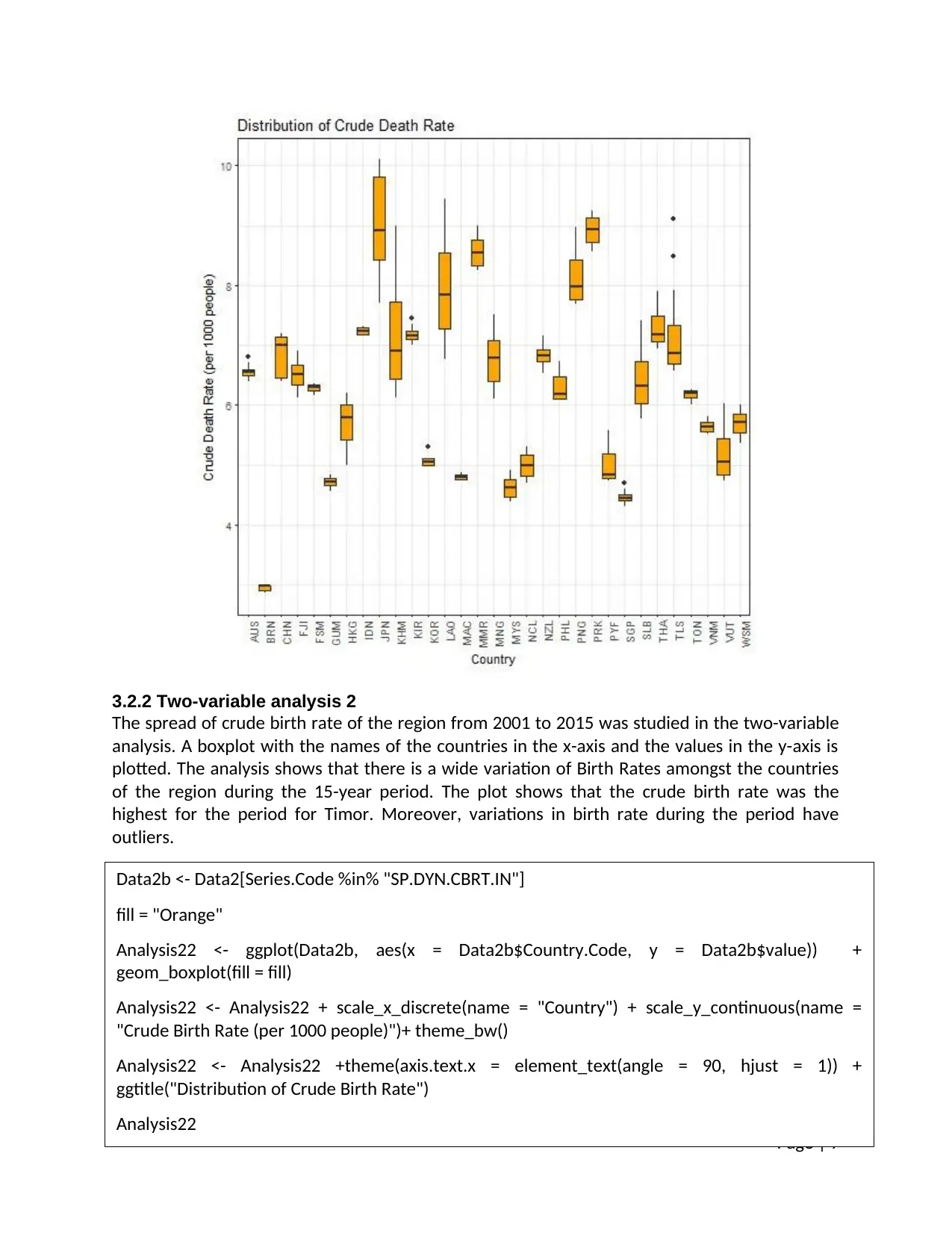
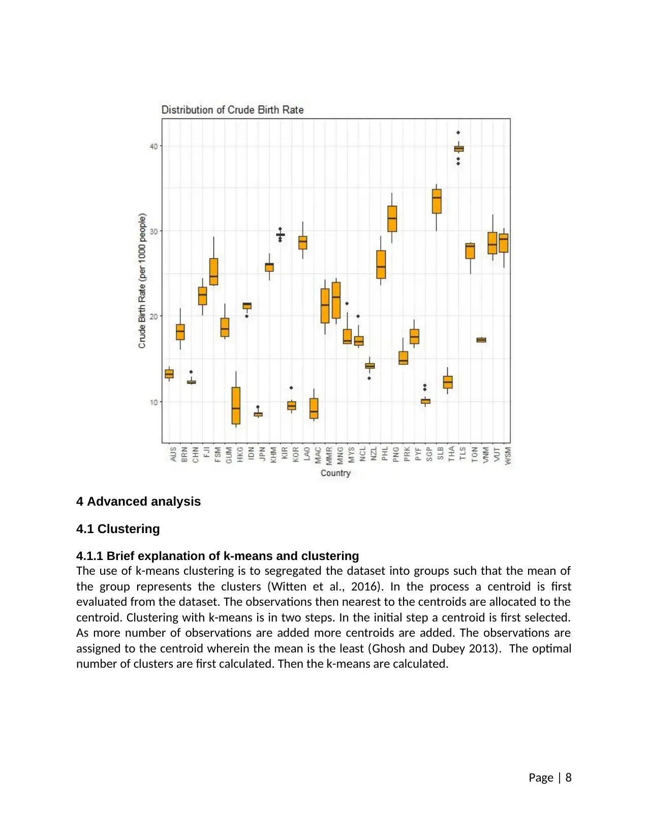
3.2.2 Two-variable analysis 2
The spread of crude birth rate of the region from 2001 to 2015 was studied in the two-variable
analysis. A boxplot with the names of the countries in the x-axis and the values in the y-axis is
plotted. The analysis shows that there is a wide variation of Birth Rates amongst the countries
of the region during the 15-year period. The plot shows that the crude birth rate was the
highest for the period for Timor. Moreover, variations in birth rate during the period have
outliers.
Page | 7
Data2b <- Data2[Series.Code %in% "SP.DYN.CBRT.IN"]
fill = "Orange"
Analysis22 <- ggplot(Data2b, aes(x = Data2b$Country.Code, y = Data2b$value)) +
geom_boxplot(fill = fill)
Analysis22 <- Analysis22 + scale_x_discrete(name = "Country") + scale_y_continuous(name =
"Crude Birth Rate (per 1000 people)")+ theme_bw()
Analysis22 <- Analysis22 +theme(axis.text.x = element_text(angle = 90, hjust = 1)) +
ggtitle("Distribution of Crude Birth Rate")
Analysis22

4 Advanced analysis
4.1 Clustering
4.1.1 Brief explanation of k-means and clustering
The use of k-means clustering is to segregated the dataset into groups such that the mean of
the group represents the clusters (Witten et al., 2016). In the process a centroid is first
evaluated from the dataset. The observations then nearest to the centroids are allocated to the
centroid. Clustering with k-means is in two steps. In the initial step a centroid is first selected.
As more number of observations are added more centroids are added. The observations are
assigned to the centroid wherein the mean is the least (Ghosh and Dubey 2013). The optimal
number of clusters are first calculated. Then the k-means are calculated.
Page | 8

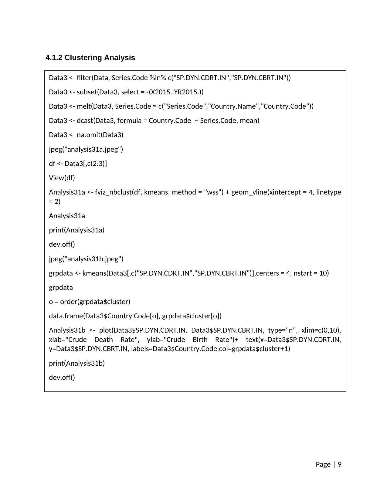
4.1.2 Clustering Analysis
Page | 9
Data3 <- filter(Data, Series.Code %in% c("SP.DYN.CDRT.IN","SP.DYN.CBRT.IN"))
Data3 <- subset(Data3, select = -(X2015..YR2015.))
Data3 <- melt(Data3, Series.Code = c("Series.Code","Country.Name","Country.Code"))
Data3 <- dcast(Data3, formula = Country.Code ~ Series.Code, mean)
Data3 <- na.omit(Data3)
jpeg("analysis31a.jpeg")
df <- Data3[,c(2:3)]
View(df)
Analysis31a <- fviz_nbclust(df, kmeans, method = "wss") + geom_vline(xintercept = 4, linetype
= 2)
Analysis31a
print(Analysis31a)
dev.off()
jpeg("analysis31b.jpeg")
grpdata <- kmeans(Data3[,c("SP.DYN.CDRT.IN","SP.DYN.CBRT.IN")],centers = 4, nstart = 10)
grpdata
o = order(grpdata$cluster)
data.frame(Data3$Country.Code[o], grpdata$cluster[o])
Analysis31b <- plot(Data3$SP.DYN.CDRT.IN, Data3$SP.DYN.CBRT.IN, type="n", xlim=c(0,10),
xlab="Crude Death Rate", ylab="Crude Birth Rate")+ text(x=Data3$SP.DYN.CDRT.IN,
y=Data3$SP.DYN.CBRT.IN, labels=Data3$Country.Code,col=grpdata$cluster+1)
print(Analysis31b)
dev.off()

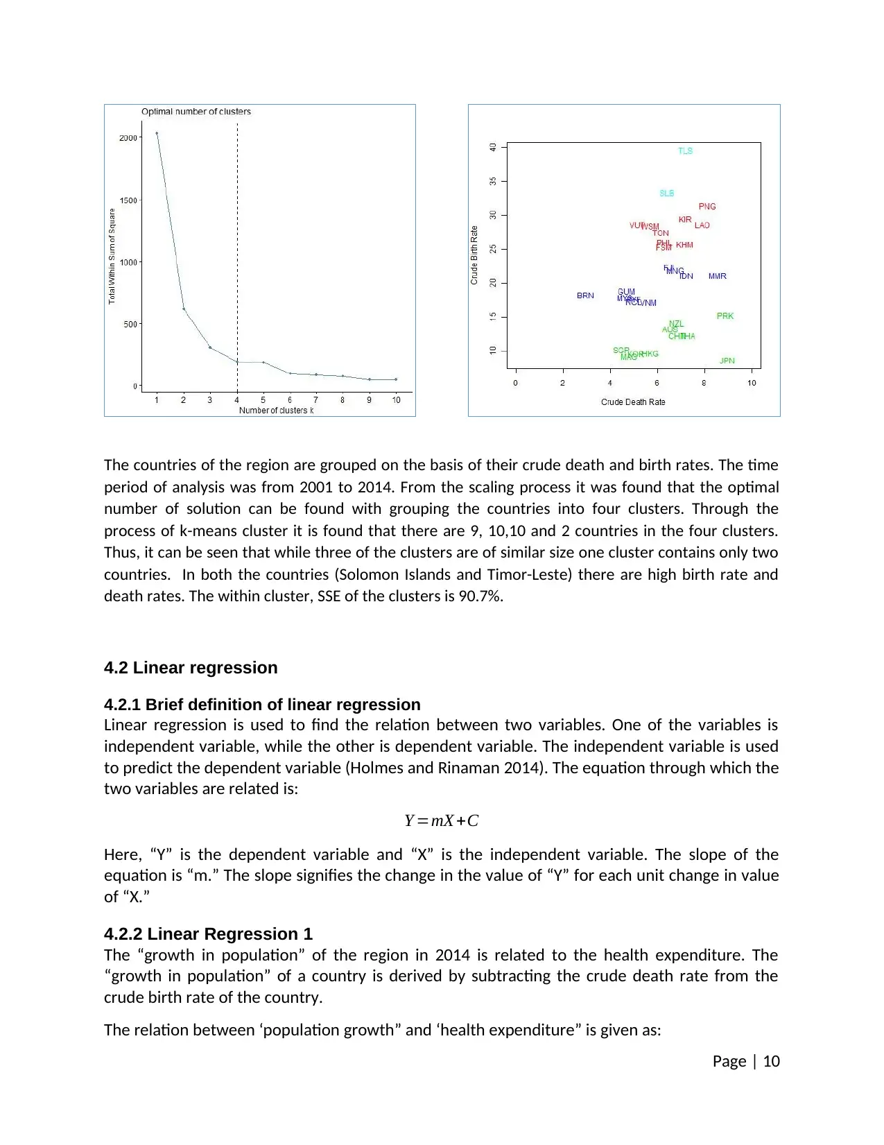
The countries of the region are grouped on the basis of their crude death and birth rates. The time
period of analysis was from 2001 to 2014. From the scaling process it was found that the optimal
number of solution can be found with grouping the countries into four clusters. Through the
process of k-means cluster it is found that there are 9, 10,10 and 2 countries in the four clusters.
Thus, it can be seen that while three of the clusters are of similar size one cluster contains only two
countries. In both the countries (Solomon Islands and Timor-Leste) there are high birth rate and
death rates. The within cluster, SSE of the clusters is 90.7%.
4.2 Linear regression
4.2.1 Brief definition of linear regression
Linear regression is used to find the relation between two variables. One of the variables is
independent variable, while the other is dependent variable. The independent variable is used
to predict the dependent variable (Holmes and Rinaman 2014). The equation through which the
two variables are related is:
Y =mX +C
Here, “Y” is the dependent variable and “X” is the independent variable. The slope of the
equation is “m.” The slope signifies the change in the value of “Y” for each unit change in value
of “X.”
4.2.2 Linear Regression 1
The “growth in population” of the region in 2014 is related to the health expenditure. The
“growth in population” of a country is derived by subtracting the crude death rate from the
crude birth rate of the country.
The relation between ‘population growth” and ‘health expenditure” is given as:
Page | 10