Population Analysis: Coursework on Population Growth and its Impacts

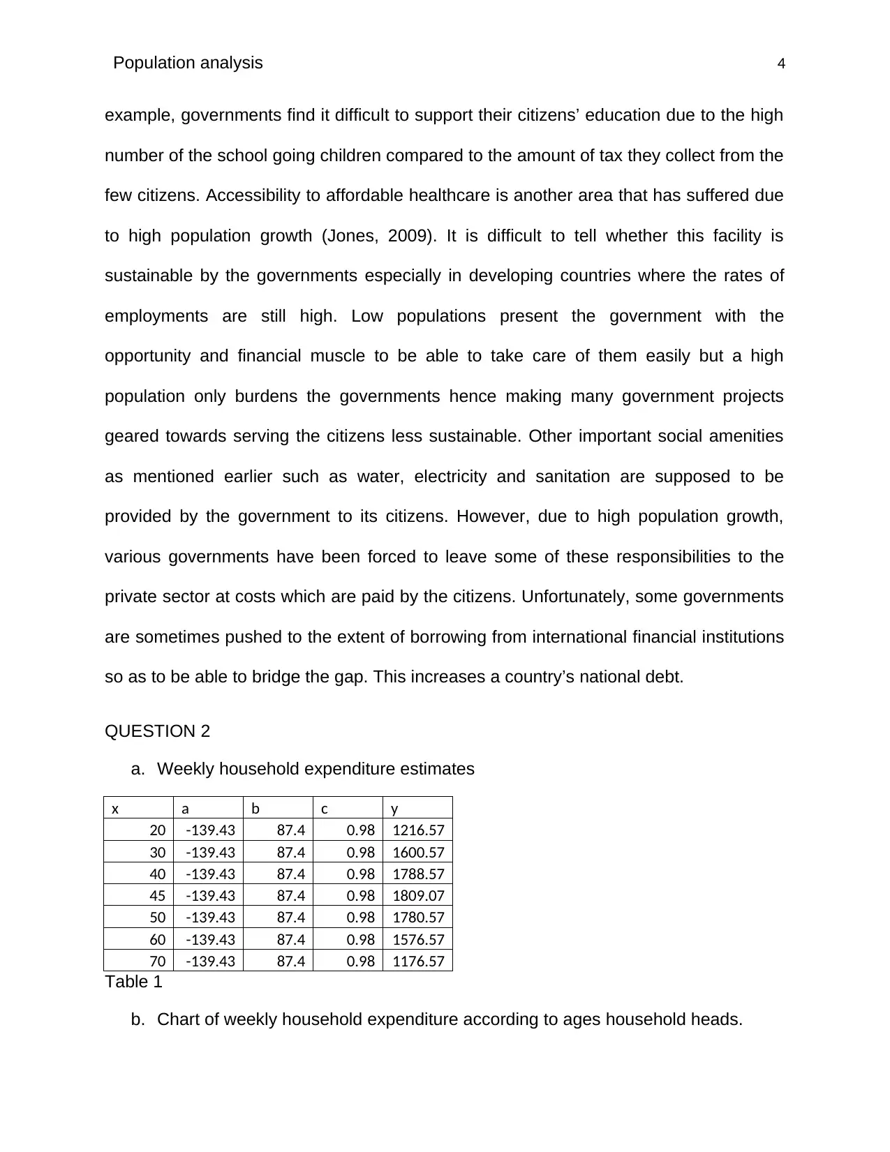
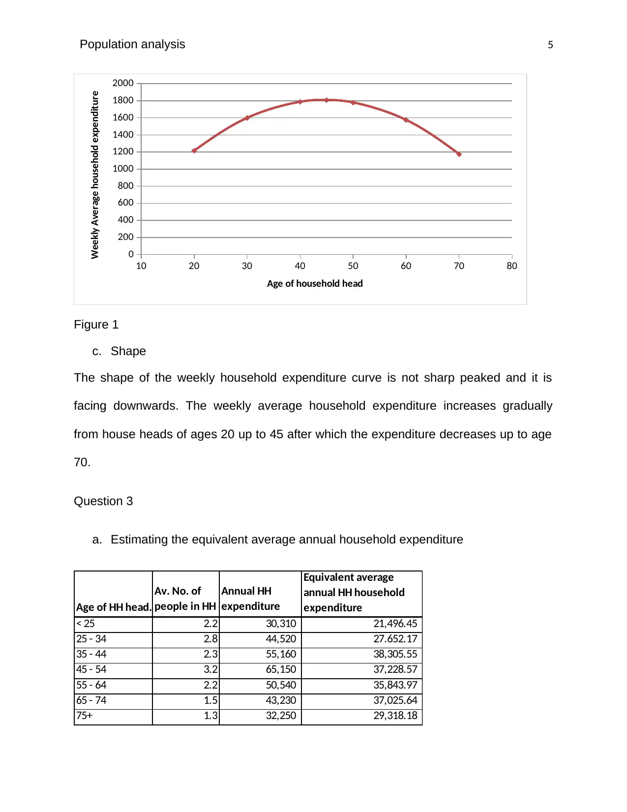
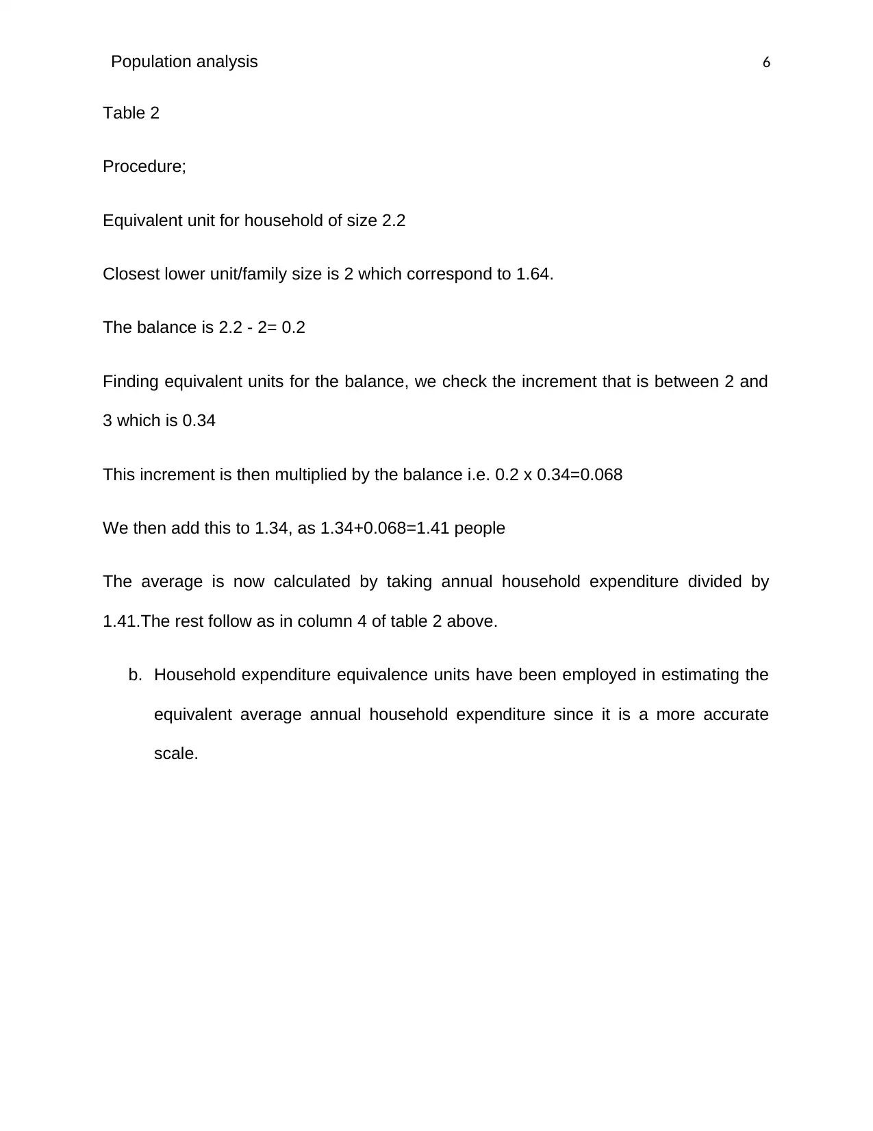
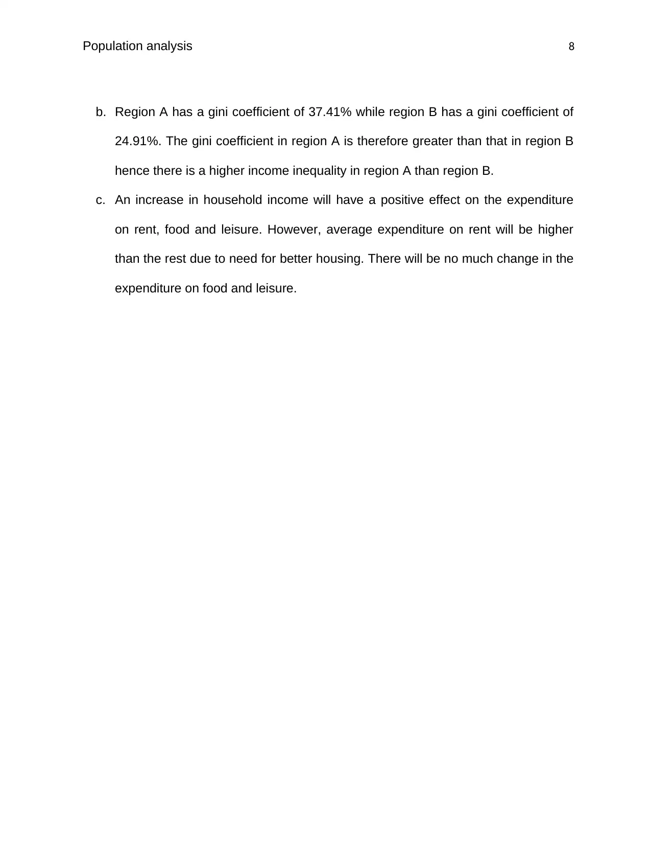
This economics assignment delves into the multifaceted impacts of population growth. It explores how rising populations affect food consumption, leading to potential shortages, price fluctuations, and health consequences. The analysis examines the relationship between population growth and income per capita, considering factors like employment rates and entrepreneurial activities. Furthermore, the assignment investigates the sustainability of resources and public services in the face of increasing population demands. The solution also includes an analysis of weekly household expenditure, its shape and estimating equivalent average annual household expenditure. Finally, it calculates and interprets the Gini coefficient for two regions, assessing income inequality and the effects of increased household income on expenditure patterns. The assignment utilizes tables, and figures to present the findings, and concludes with a list of relevant references.

Population analysis 1
Student name:
Student ID:
Course Code:

Population analysis 2
Question one
Impacts of population growth on food consumption, income per capita growth,
and sustainability
Population growth has various impacts on such responses as food consumption,
sustainability and income per capita.
High population growth leads to overstretched resources one of them being land. As it is
known, land is neither movable nor elastic. The amount of land remains constant as
population grows from decade to decade. This forces the population to encroach on
lands that are either preserved for agriculture so as to have locations for settlement.
This in turn leads to less food production hence leading to food shortage in the market.
The high demand for food consequently causes the plummeting of food prices. The
resultant effect is poor health and malnutrition among the population that are not able to
afford the food in the market. High population growth also encourages rural urban
migration (Gradstein, 2012). Many young and energetic people leave the rural areas
which are agriculturally rich in search of jobs in the urban areas because of
fragmentation of land in the rural areas due to high population which they would have
rather used to practice agriculture and support their lives (Bruckner, 2012). The result of
this is less food production in the rural areas since the young and energetic that would
have remained to practice agriculture and produce have migrated to the urban areas in
search of white collar jobs. High food demand has forced nations to spend huge
amounts of their budgets to import food from other countries to supplement their
production.

Population analysis 3
Per capita income is the annual average income of a nation per head. This variable has
a great correlation or relationship with population growth. High population growth means
that the population is growing at a high rate. This can be very detrimental especially if
this is happening at the expense of employment opportunities or income generating
activities. When the rate of population becomes higher than the rate of job opportunities,
it means not all members of the population will get to be employed (Caldwell, 2016).
The rate of unemployment will be as high as the rate of population growth if the
numbers of job opportunities remain constant. The per capita will be reduced since the
number of people who are working and earning are less compared to those who are
unemployed or not earning since this value is calculated as an average on all
individuals whether working and earning or not. However, there can be cases of high
population and high employment rate yet the per capita income remains low. This
happens when a high competition for job opportunities causes the employers to take
advantage of the high demand to lower the salaries that they offer for their various
opportunities thus leading to lower per capita (Deaton, 2007). High population growth on
the other hand can also lead to high per capita income. This happens when the
population instead of looking for employment decides to take advantage of the high
population and venture into entrepreneurship. This will lead to a high population being
able to earn income thus raising the countries per capita income.
Population growth can also be said to have profound impacts on sustainability of
various resources that are supposed to serve the population. High population has been
found to overstretch facilities such as hospitals, schools, water, electricity and other
public utilities that are provided by a government to its citizens (Henderson, 2013). For

Population analysis 4
example, governments find it difficult to support their citizens’ education due to the high
number of the school going children compared to the amount of tax they collect from the
few citizens. Accessibility to affordable healthcare is another area that has suffered due
to high population growth (Jones, 2009). It is difficult to tell whether this facility is
sustainable by the governments especially in developing countries where the rates of
employments are still high. Low populations present the government with the
opportunity and financial muscle to be able to take care of them easily but a high
population only burdens the governments hence making many government projects
geared towards serving the citizens less sustainable. Other important social amenities
as mentioned earlier such as water, electricity and sanitation are supposed to be
provided by the government to its citizens. However, due to high population growth,
various governments have been forced to leave some of these responsibilities to the
private sector at costs which are paid by the citizens. Unfortunately, some governments
are sometimes pushed to the extent of borrowing from international financial institutions
so as to be able to bridge the gap. This increases a country’s national debt.
QUESTION 2
a. Weekly household expenditure estimates
x a b c y
20 -139.43 87.4 0.98 1216.57
30 -139.43 87.4 0.98 1600.57
40 -139.43 87.4 0.98 1788.57
45 -139.43 87.4 0.98 1809.07
50 -139.43 87.4 0.98 1780.57
60 -139.43 87.4 0.98 1576.57
70 -139.43 87.4 0.98 1176.57
Table 1
b. Chart of weekly household expenditure according to ages household heads.

Population analysis 5
10 20 30 40 50 60 70 80
0
200
400
600
800
1000
1200
1400
1600
1800
2000
Age of household head
Weekly Average household expenditure
Figure 1
c. Shape
The shape of the weekly household expenditure curve is not sharp peaked and it is
facing downwards. The weekly average household expenditure increases gradually
from house heads of ages 20 up to 45 after which the expenditure decreases up to age
70.
Question 3
a. Estimating the equivalent average annual household expenditure
Age of HH head.
Av. No. of
people in HH
Annual HH
expenditure
Equivalent average
annual HH household
expenditure
< 25 2.2 30,310 21,496.45
25 - 34 2.8 44,520 27.652.17
35 - 44 2.3 55,160 38,305.55
45 - 54 3.2 65,150 37,228.57
55 - 64 2.2 50,540 35,843.97
65 - 74 1.5 43,230 37,025.64
75+ 1.3 32,250 29,318.18

Population analysis 6
Table 2
Procedure;
Equivalent unit for household of size 2.2
Closest lower unit/family size is 2 which correspond to 1.64.
The balance is 2.2 - 2= 0.2
Finding equivalent units for the balance, we check the increment that is between 2 and
3 which is 0.34
This increment is then multiplied by the balance i.e. 0.2 x 0.34=0.068
We then add this to 1.34, as 1.34+0.068=1.41 people
The average is now calculated by taking annual household expenditure divided by
1.41.The rest follow as in column 4 of table 2 above.
b. Household expenditure equivalence units have been employed in estimating the
equivalent average annual household expenditure since it is a more accurate
scale.

Population analysis 7
Question 4
a. Gini coefficient
REGION A
No. of
household
xi+1-
xi Average weekly exp. On rent
No. of families x
average yi+1-yi
(xi+1-xi)(yi+1-
yi)
105 21 200 21000 10.71 224.91
120 24 300 36000 39.79 954.96
80 16 400 32000 74.49 1191.84
100 20 500 50000 87.24 1744.8
95 19 600 57000
112.7
5 2142.25
500 2000 196000 6258.76
Table 2
Gini coefficient for region A
Gini coefficient =100 %−∑ ( yi +1+ yi )( xi+1−xi )/100
¿ 100 %−( 6258.76
100 )
¿ 37.41 %
Gini- coefficient for region B
REGION B
No. of
household
xi+1-
xi Average weekly exp. On rent
No. of fam x
average yi+1-yi
(xi+1-xi)(yi+1-
yi)
30 6 200 6000 2.5 15
55 11 300 16500 11.8 129.8
75 15 400 30000 28.54 428.1
150 30 500 75000 65.22 1956.6
190 38 600 114000
131.0
5 4979.9
500 2000 241500 7509.4
Table 3
Gini coefficient =100 %−∑ ( yi +1+ yi )( xi+1−xi )/100
¿ 100 %−( 7509.4
100 )
¿ 24.91 %

Population analysis 8
b. Region A has a gini coefficient of 37.41% while region B has a gini coefficient of
24.91%. The gini coefficient in region A is therefore greater than that in region B
hence there is a higher income inequality in region A than region B.
c. An increase in household income will have a positive effect on the expenditure
on rent, food and leisure. However, average expenditure on rent will be higher
than the rest due to need for better housing. There will be no much change in the
expenditure on food and leisure.

Population analysis 9
References
Bruckner, M. (2012)."Economic Growth, Size of the Agriculture al Sector, and
Urbanization in Africa." Journal of Urban Economics 71: 26-36.
Bruckner, M., A. Chong, and M. Gradstein (2012). "Estimating the Permanent Income
Elasticity of Government Spending: Evidence on Wagner's Law Based on Oil Price
Shocks." Journal of Public Economics 96: 1025-1034.
Caldwell, J. (2016). “Toward a Restatement of Demographic Transition Theory.”
Population and Development Review, 2(3/4)
Deaton, A. (2007). “Global patterns of income and health: facts, interpretations and
policies.”
Henderson, V. (2013). "The Urbanization Process and Economic Growth: The So-What
Question." Journal of Economic Growth 8: 47-71.
Jones, C. (2009). Growth and Ideas. Handbook of Economic Growth, Volume 1B,
Chapter 16. Edited by Philippe Aghion and Steven N. Durlauf.