Computer Controlled Systems: Assignment 2 - Position Control Design

This assignment solution addresses the analysis and control design of a position control system. The solution begins by converting the system into a state-space format and simulating its response to a unit step input. It then discretizes the system and investigates the impact of different sampling times using MATLAB simulations. The core of the assignment involves designing a state variable feedback regulator to achieve desired performance characteristics, specifically placing complex poles at specified locations. The closed-loop system's response is then simulated and compared to the original system. The solution also explores the design of a dead-beat observer to provide state variables when direct measurements are unavailable, simulating the complete system with the regulator and observer in place.

Running head: ASSIGNMENT 2
ASSIGNMENT 2
Name of the Student
Name of the University
Author Note

1ASSIGNMENT 2
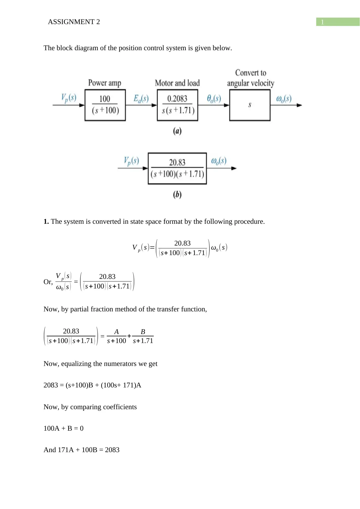
The block diagram of the position control system is given below.
1. The system is converted in state space format by the following procedure.
V p (s)= ( 20.83
( s+ 100 ) ( s+ 1.71 ) )ω0 (s)
Or, V p ( s )
ω0 ( s ) = ( 20.83
( s +100 ) ( s +1.71 ) )
Now, by partial fraction method of the transfer function,
( 20.83
( s +100 ) ( s +1.71 ) ) = A
s +100 + B
s+1.71
Now, equalizing the numerators we get
2083 = (s+100)B + (100s+ 171)A
Now, by comparing coefficients
100A + B = 0
And 171A + 100B = 2083

2ASSIGNMENT 2
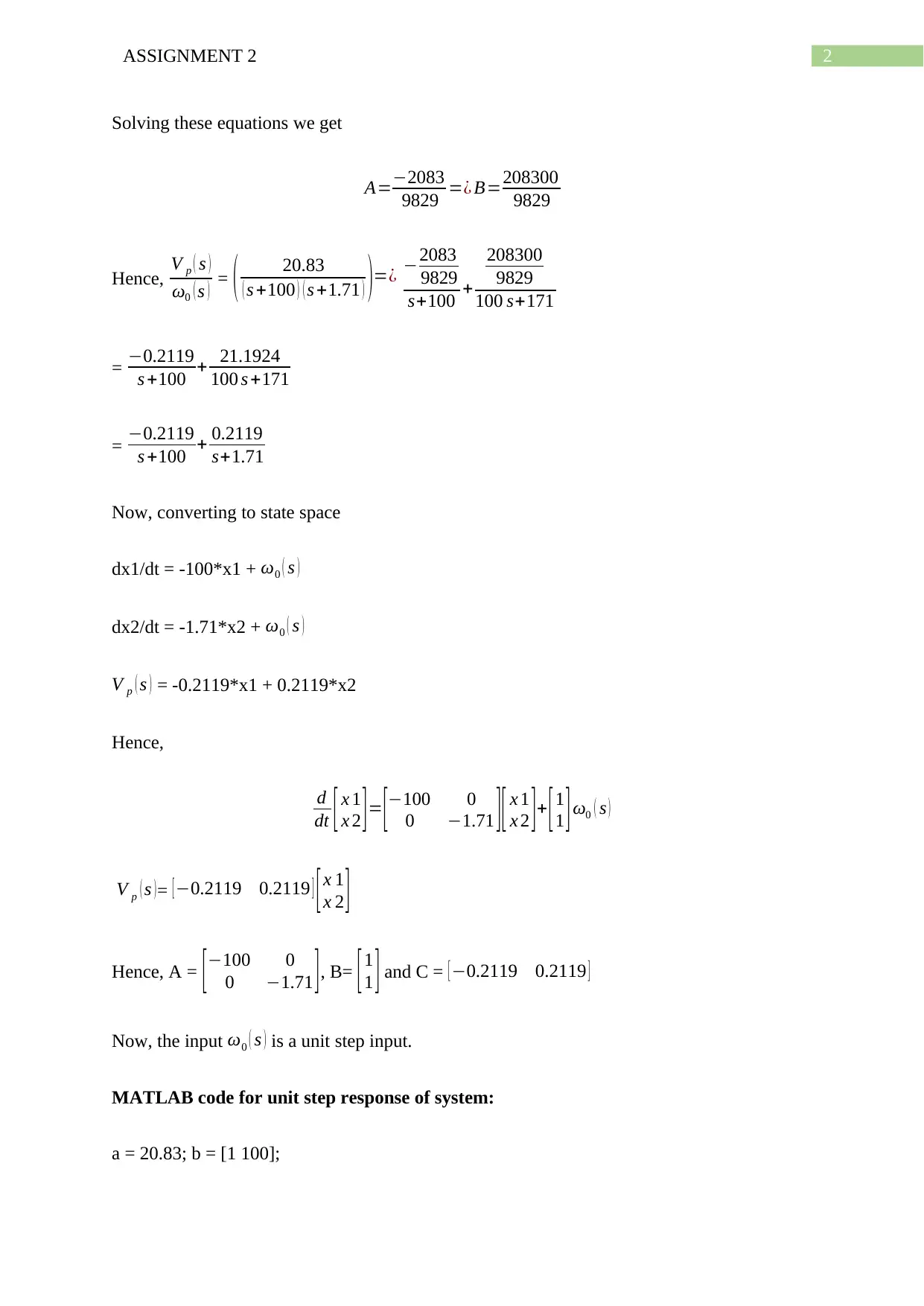
Solving these equations we get
A=−2083
9829 =¿ B=208300
9829
Hence, V p ( s )
ω0 ( s ) = ( 20.83
( s +100 ) ( s +1.71 ) )=¿ −2083
9829
s+100 +
208300
9829
100 s+171
= −0.2119
s +100 + 21.1924
100 s +171
= −0.2119
s +100 + 0.2119
s+1.71
Now, converting to state space
dx1/dt = -100*x1 + ω0 ( s )
dx2/dt = -1.71*x2 + ω0 ( s )
V p ( s ) = -0.2119*x1 + 0.2119*x2
Hence,
d
dt [ x 1
x 2 ] = [−100 0
0 −1.71 ][ x 1
x 2 ] + [ 1
1 ] ω0 ( s )
V p ( s )= [−0.2119 0.2119 ] [x 1
x 2 ]
Hence, A = [ −100 0
0 −1.71 ], B= [ 1
1 ] and C = [ −0.2119 0.2119 ]
Now, the input ω0 ( s ) is a unit step input.
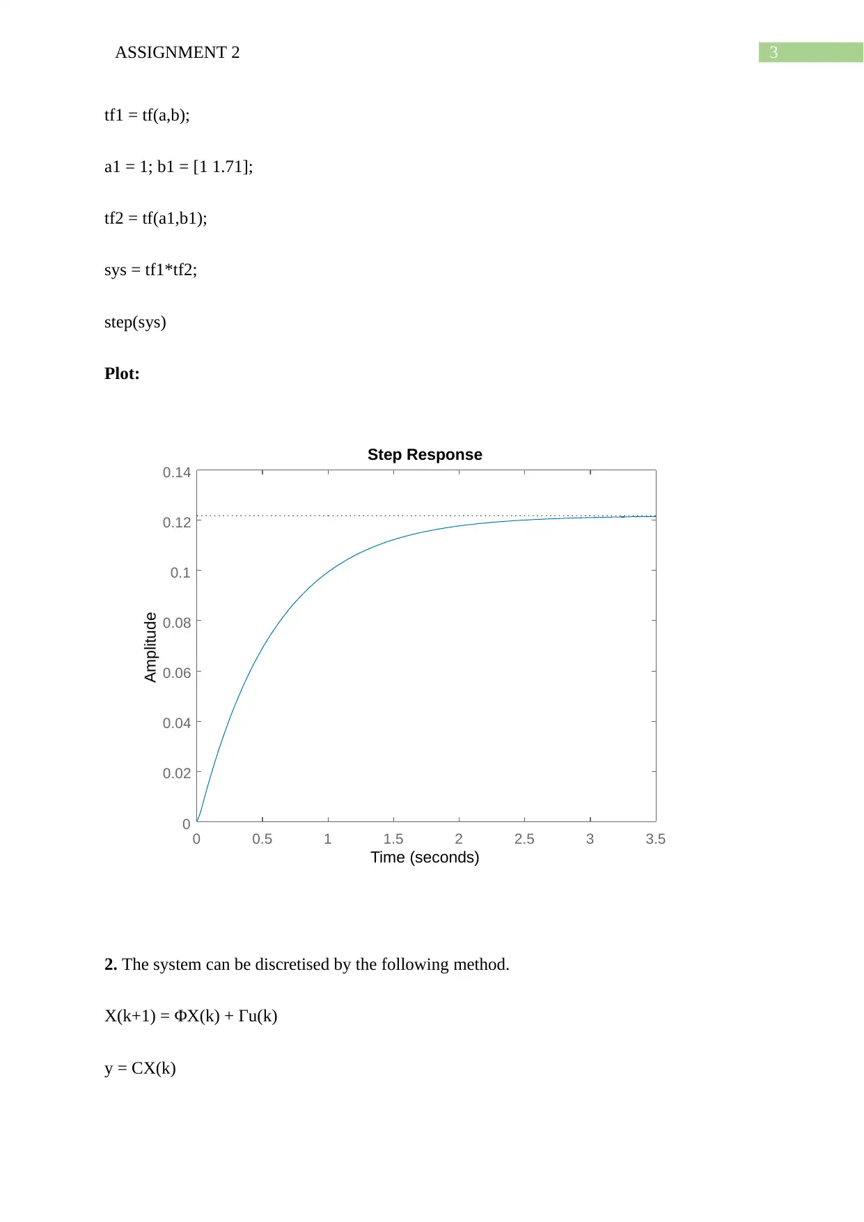
MATLAB code for unit step response of system:
a = 20.83; b = [1 100];

3ASSIGNMENT 2
tf1 = tf(a,b);
a1 = 1; b1 = [1 1.71];
tf2 = tf(a1,b1);
sys = tf1*tf2;
step(sys)
Plot:
0 0.5 1 1.5 2 2.5 3 3.5
0
0.02
0.04
0.06
0.08
0.1
0.12
0.14
Step Response
Time (seconds)
Amplitude
2. The system can be discretised by the following method.
X(k+1) = ΦX(k) + Γu(k)
y = CX(k)

4ASSIGNMENT 2
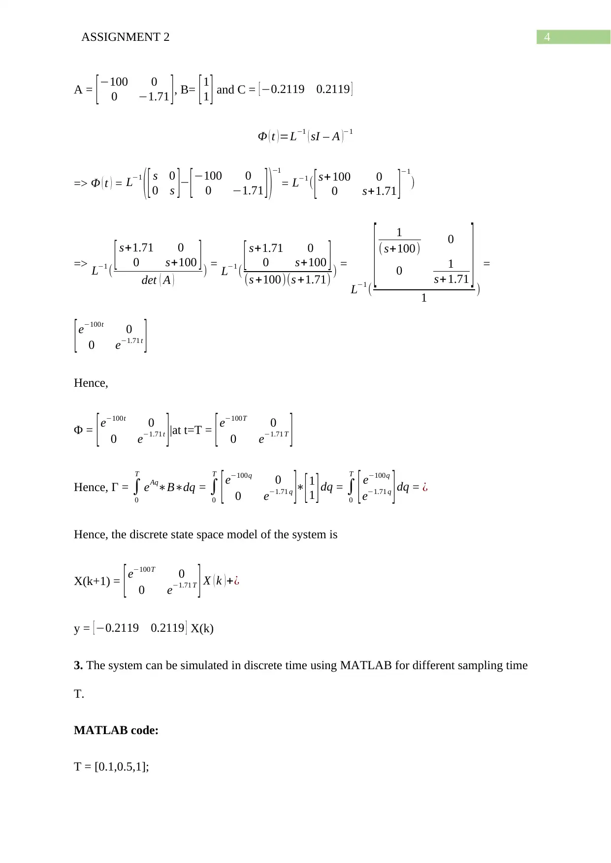
A = [ −100 0
0 −1.71 ], B= [1
1 ] and C = [ −0.2119 0.2119 ]
Φ ( t )=L−1 ( sI – A )−1
=> Φ ( t ) = L−1
( [ s 0
0 s ]− [ −100 0
0 −1.71 ] )
−1
= L−1 ( [s+100 0
0 s+1.71 ]−1
)
=> L−1 ( [ s+1.71 0
0 s+100 ]
det ( A ) ) = L−1 ( [ s+1.71 0
0 s+100 ]
(s +100)(s +1.71) ) =
L−1 (
[ 1
(s+100) 0
0 1
s+1.71 ]1 )
=
[e−100t 0
0 e−1.71 t ]
Hence,
Φ = [ e−100t 0
0 e−1.71 t ]|at t=T = [ e−100T 0
0 e−1.71 T ]
Hence, Γ = ∫
0
T
eAq∗B∗dq = ∫
0
T
[e−100q 0
0 e−1.71 q ]∗
[1
1 ]dq = ∫
0
T
[ e−100q
e−1.71 q ] dq = ¿
Hence, the discrete state space model of the system is
X(k+1) = [e−100T 0
0 e−1.71 T ] X ( k )+¿
y = [ −0.2119 0.2119 ] X(k)
3. The system can be simulated in discrete time using MATLAB for different sampling time
T.
MATLAB code:
T = [0.1,0.5,1];

5ASSIGNMENT 2
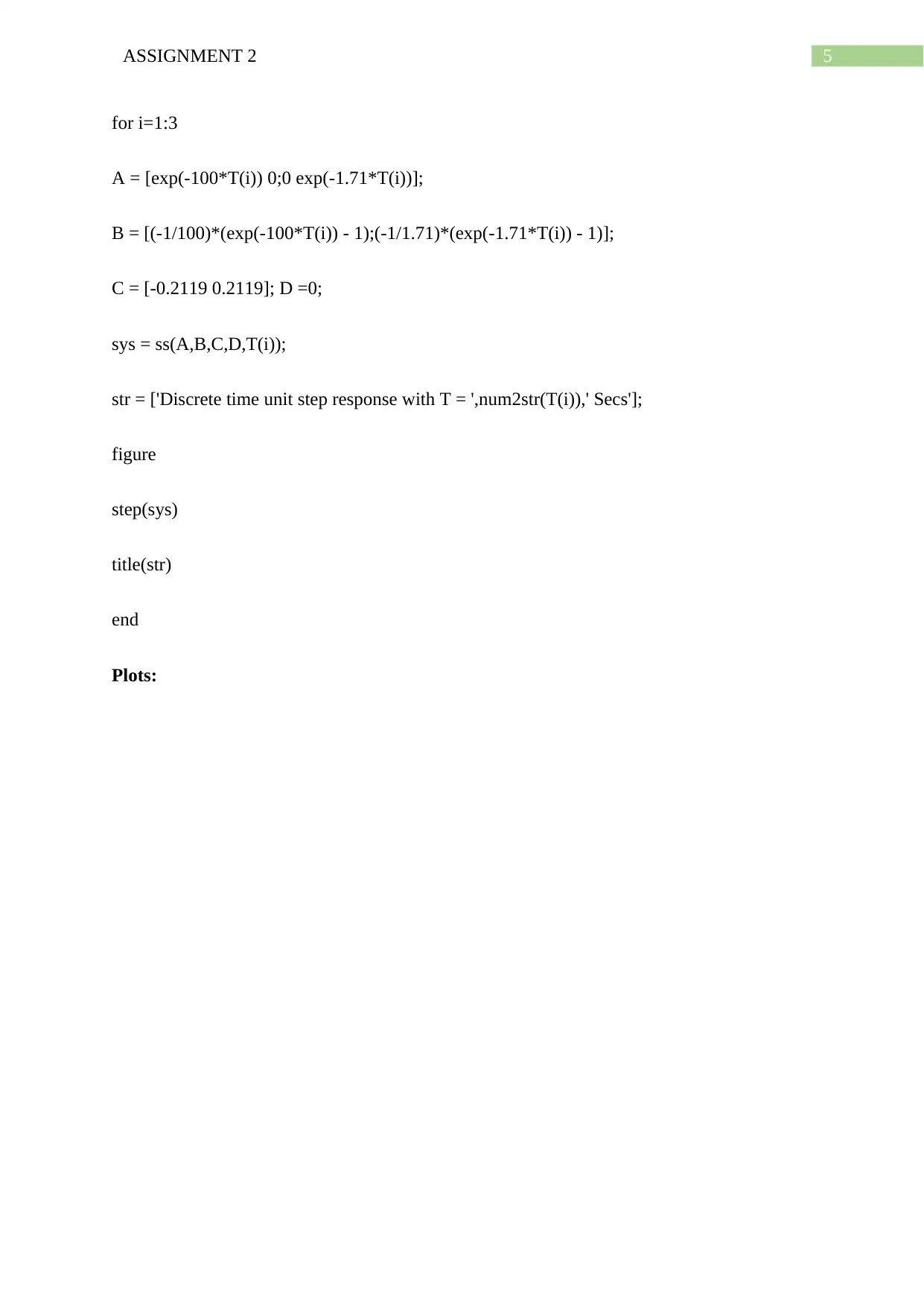
for i=1:3
A = [exp(-100*T(i)) 0;0 exp(-1.71*T(i))];
B = [(-1/100)*(exp(-100*T(i)) - 1);(-1/1.71)*(exp(-1.71*T(i)) - 1)];
C = [-0.2119 0.2119]; D =0;
sys = ss(A,B,C,D,T(i));
str = ['Discrete time unit step response with T = ',num2str(T(i)),' Secs'];
figure
step(sys)
title(str)
end
Plots:

6ASSIGNMENT 2
0 0.5 1 1.5 2 2.5 3 3.5
0
0.02
0.04
0.06
0.08
0.1
0.12
0.14
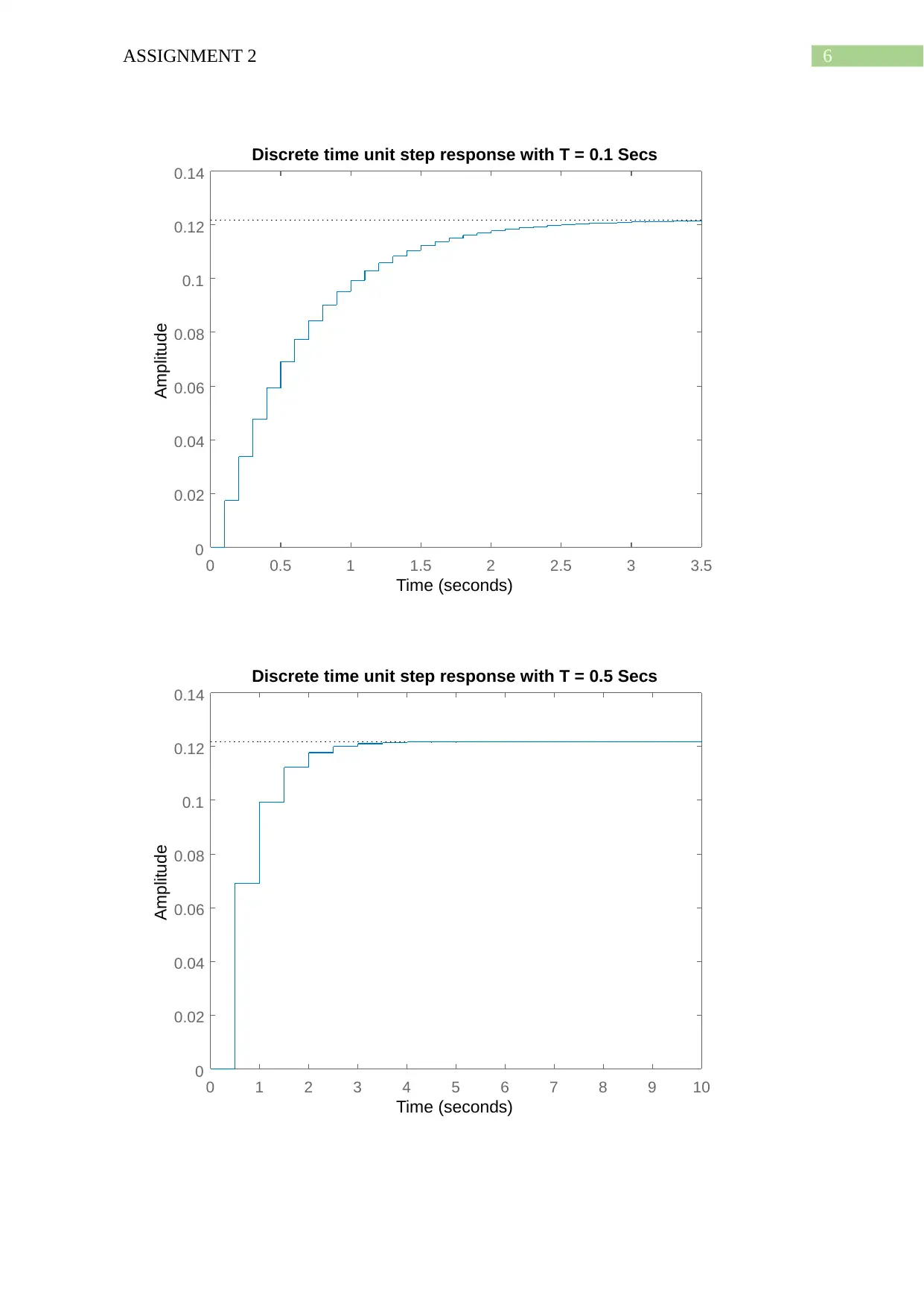
Discrete time unit step response with T = 0.1 Secs
Time (seconds)
Amplitude
0 1 2 3 4 5 6 7 8 9 10
0
0.02
0.04
0.06
0.08
0.1
0.12
0.14
Discrete time unit step response with T = 0.5 Secs
Time (seconds)
Amplitude

7ASSIGNMENT 2
0 2 4 6 8 10 12 14 16 18 20
0
0.02
0.04
0.06
0.08
0.1
0.12
0.14
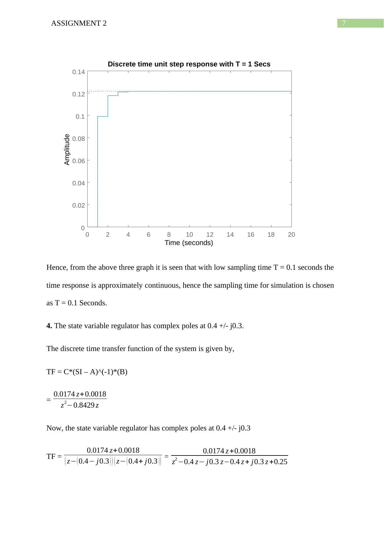
Discrete time unit step response with T = 1 Secs
Time (seconds)
Amplitude
Hence, from the above three graph it is seen that with low sampling time T = 0.1 seconds the
time response is approximately continuous, hence the sampling time for simulation is chosen
as T = 0.1 Seconds.
4. The state variable regulator has complex poles at 0.4 +/- j0.3.
The discrete time transfer function of the system is given by,
TF = C*(SI – A)^(-1)*(B)
= 0.0174 z+0.0018
z2−0.8429 z
Now, the state variable regulator has complex poles at 0.4 +/- j0.3
TF = 0.0174 z+0.0018
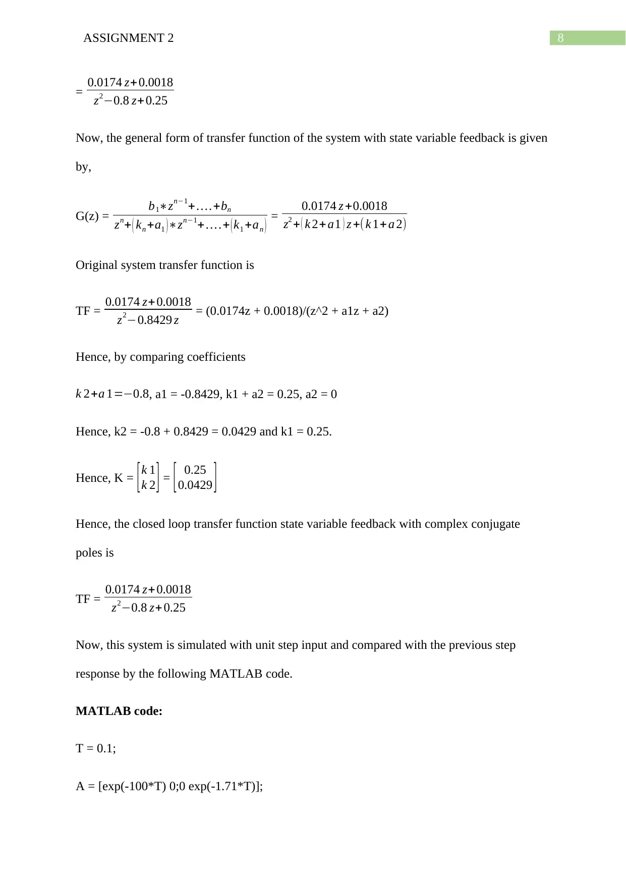
( z− ( 0.4− j0.3 ) ) ( z− ( 0.4+ j0.3 ) ) = 0.0174 z +0.0018
z2 −0.4 z− j0.3 z−0.4 z + j0.3 z +0.25

8ASSIGNMENT 2
= 0.0174 z+0.0018
z2−0.8 z+ 0.25
Now, the general form of transfer function of the system with state variable feedback is given
by,
G(z) = b1∗zn−1+ … .+bn
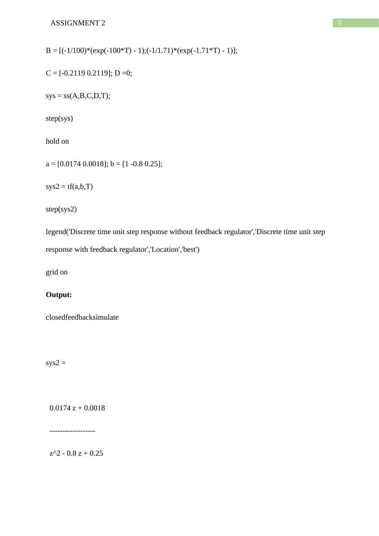
zn+ ( kn +a1 )∗zn−1+ … .+ ( k1 +an ) = 0.0174 z +0.0018
z2 + ( k 2+ a1 ) z +( k 1+ a 2)
Original system transfer function is
TF = 0.0174 z+0.0018
z2−0.8429 z = (0.0174z + 0.0018)/(z^2 + a1z + a2)
Hence, by comparing coefficients
k 2+a 1=−0.8, a1 = -0.8429, k1 + a2 = 0.25, a2 = 0
Hence, k2 = -0.8 + 0.8429 = 0.0429 and k1 = 0.25.
Hence, K = [ k 1
k 2 ] = [ 0.25
0.0429 ]
Hence, the closed loop transfer function state variable feedback with complex conjugate
poles is
TF = 0.0174 z+0.0018
z2−0.8 z+ 0.25
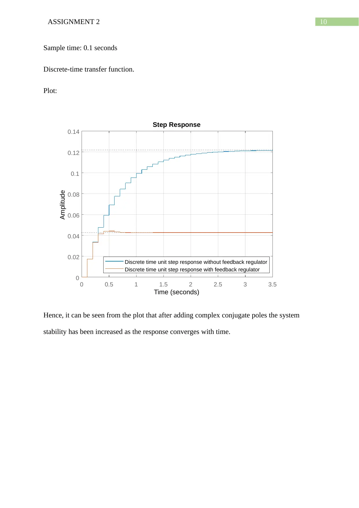
Now, this system is simulated with unit step input and compared with the previous step
response by the following MATLAB code.
MATLAB code:
T = 0.1;
A = [exp(-100*T) 0;0 exp(-1.71*T)];

9ASSIGNMENT 2
B = [(-1/100)*(exp(-100*T) - 1);(-1/1.71)*(exp(-1.71*T) - 1)];
C = [-0.2119 0.2119]; D =0;
sys = ss(A,B,C,D,T);
step(sys)
hold on
a = [0.0174 0.0018]; b = [1 -0.8 0.25];
sys2 = tf(a,b,T)
step(sys2)
legend('Discrete time unit step response without feedback regulator','Discrete time unit step
response with feedback regulator','Location','best')
grid on
Output:
closedfeedbacksimulate
sys2 =
0.0174 z + 0.0018
------------------
z^2 - 0.8 z + 0.25

10ASSIGNMENT 2
Sample time: 0.1 seconds
Discrete-time transfer function.
Plot:
0 0.5 1 1.5 2 2.5 3 3.5
0
0.02
0.04
0.06
0.08
0.1
0.12
0.14
Discrete time unit step response without feedback regulator
Discrete time unit step response with feedback regulator
Step Response
Time (seconds)
Amplitude
Hence, it can be seen from the plot that after adding complex conjugate poles the system
stability has been increased as the response converges with time.