Software Processes Analysis: Curve Fitting Models and Techniques

This assignment delves into the application of curve fitting techniques within software processes, examining various models such as general polynomial and general linear fit. It explores the use of predictive analysis to interpret results and make informed decisions, covering data inspection, cleaning, and transformation. The assignment highlights the importance of selecting appropriate analysis techniques and discusses the learning and testing phases involved in model development. It also compares different models based on their efficiency and suitability for various scenarios, along with the time taken for implementation. Furthermore, the assignment emphasizes the similarities between operating datasets and highlights the importance of knowledge encoding techniques. The analysis includes references to relevant sources, providing a comprehensive understanding of the topic and its practical applications.

Software
Processes

Table of Contents
1. Question 1................................................................................................................................2
1.1 Models Used.....................................................................................................................2
1.2 Analysis Technique Used..................................................................................................3
1.3 Reasons for Choosing Analysis Technique......................................................................4
2. Question 2................................................................................................................................4
2.1 Model Fits- General Polynomial.......................................................................................4
2.2 Curve fitting......................................................................................................................5
3. Question 3................................................................................................................................6
3.1 Learning phase..................................................................................................................6
3.2 Testing phase.....................................................................................................................7
4. Question 4................................................................................................................................7
5. Question 5................................................................................................................................8
6. Question 6................................................................................................................................8

1. Question 1
The curve fitting models are used as it fits the requirements. It has many models and they are
described below.
Curve Fitting techniques and Models
The linear fit, Gaussian peak fit, exponential fit, power fit and logarithm fit models are used to
compute the curve fitting function in mathematical format. In addition, the following VIs used to
analyze and compute the curve fitting function. There are given below,
1) General Linear Fit VI
2) General Polynomial VI
3) Nonlinear Curve Fit VI
4) Cubic Spline Fit VI
In this General Linear Fit VI and General Polynomial VI is used for implementation work. Those
two models are described below.
The values taken for a, b and c are constant values. The graph is generated according to the
requirements. MS-EXCEL is the software tool used for implementing the curve.
1.1 Models Used
General Polynomial Fit
Use of common polynomial fit VI in curve fitting, fits data set to polynomial. The overall form
of the polynomial fit model is,
F(x) =a+bx+cx2+…..
The user initially need to set polynomial input when use the polynomial model fit VI. The
polynomial order could not assure good fitting output and it can cause oscillation. The lower
polynomial order can fulfill the best applications. Default value of the polynomial order is 2.
General Linear Fit

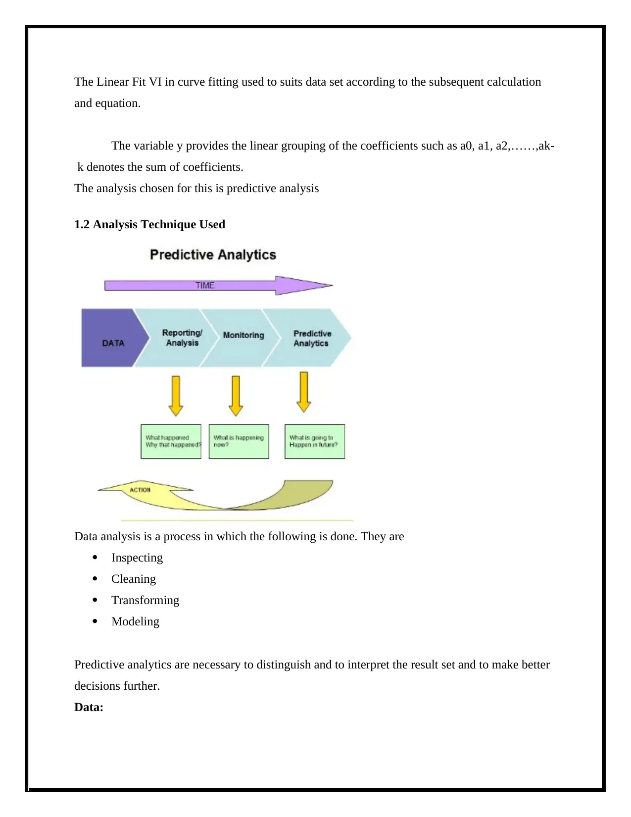
The Linear Fit VI in curve fitting used to suits data set according to the subsequent calculation
and equation.
The variable y provides the linear grouping of the coefficients such as a0, a1, a2,……,ak-
k denotes the sum of coefficients.
The analysis chosen for this is predictive analysis
1.2 Analysis Technique Used
Data analysis is a process in which the following is done. They are
 Inspecting
 Cleaning
 Transforming
 Modeling
Predictive analytics are necessary to distinguish and to interpret the result set and to make better
decisions further.
Data:

The good data is needed to perform the process of analysis. The attributes in dataset are
analyzed
Statistics:
For the statistics, the regression analysis is used. The statistical process are analyzed by
using the statistics. The effects in variable are examined and the analysis report is made for
further investigation
Assumptions:
The assumptions needs to be monitored and the predictive analysis is done for the
dataset. More attention is given the secondary variables and the external variables. The dataset
relationship is assumed, identified and is examined in better way. The assumptions are then
validated from multiple resource and modified accordingly.
1.3 Reasons for Choosing Analysis Technique
The analysis chosen for this is predictive analysis. This is because
 This is chosen as it to perform the process of analysis in better way.
 Suitable procedures related to requirements are followed in predictive analysis
 The effects in variable are examined and the analysis report is made effectively.
 In predictive analysis, the dataset relationship is assumed, identified and is
examined in better way. (Oravecz & Muth, 2017)
2. Question 2
.
The best fit model is provided below.
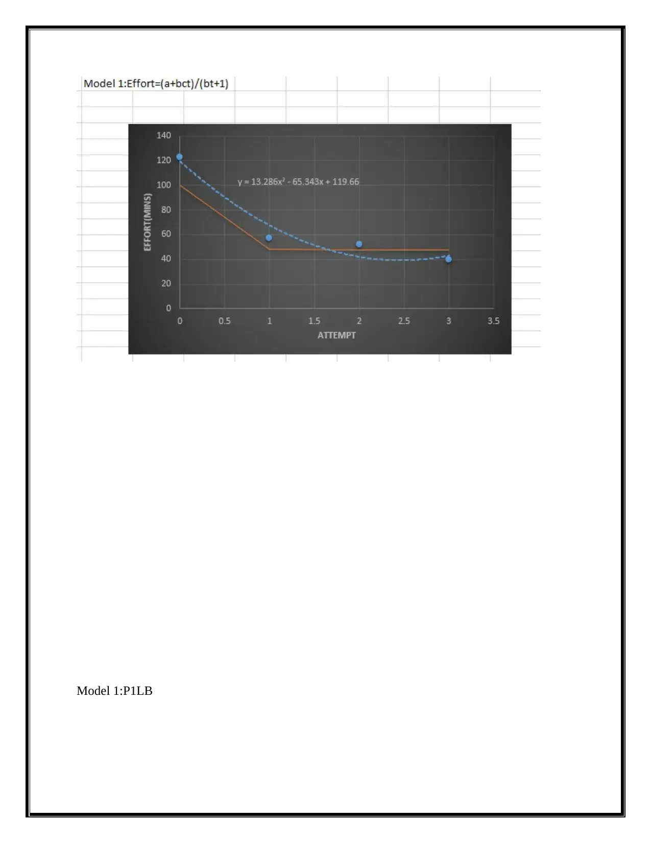
Model 1: Effort = (a + bct) / (bt +1)
The above model fits well for the set of programs in generating P1LA, P2LA, P1LB.
General polynomial is used because it uses common polynomial function in curve fitting
technique. The general description for General polynomial is provided below.

2.1 Model Fits- General Polynomial
The uses of common polynomial fit VI in curve fitting, fits data set to a polynomial function.
The over-all form of the polynomial fit model is,
F(x) =a+bx+cx2+…..
The user initially needs to set the polynomial order input when use the polynomial model fit VI.
The higher polynomial order could not assure a good fitting output and it can be a reason for
oscillation. The lower polynomial order satisfies the best applications. The default value of the
polynomial order is 2. ("Curve Fitting and Method of Least Squares | eMathZone", 2017)
The plots are provided in this.
Learning of curve fitting from the previous projects helped in summarizing the curve fitting in
different way. The new of understanding curve fitting is provided below.
2.2 Curve Fitting Technique
Generally, the curve fitting is used to find a mathematical function which is represented as f(x) in
a function class ɵ for the statistics ("Curve Fitting Software | NCSS Statistical Software | NCSS",
2017)
The below graph is generated from the dataset-

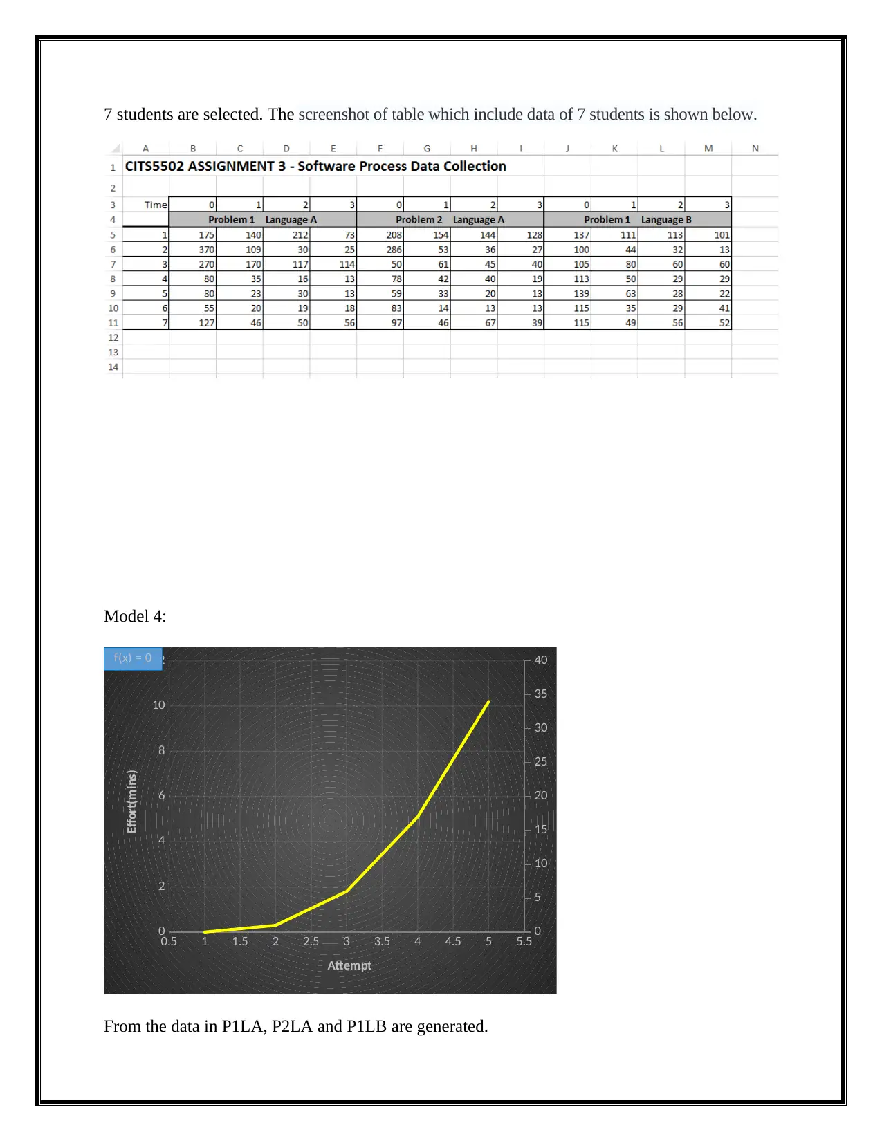
7 students are selected. The screenshot of table which include data of 7 students is shown below.
Model 4:
0.5 1 1.5 2 2.5 3 3.5 4 4.5 5 5.5
0
2
4
6
8
10
12
0
5
10
15
20
25
30
35
40f(x) = 0
Attempt
Effort(mins)
From the data in P1LA, P2LA and P1LB are generated.

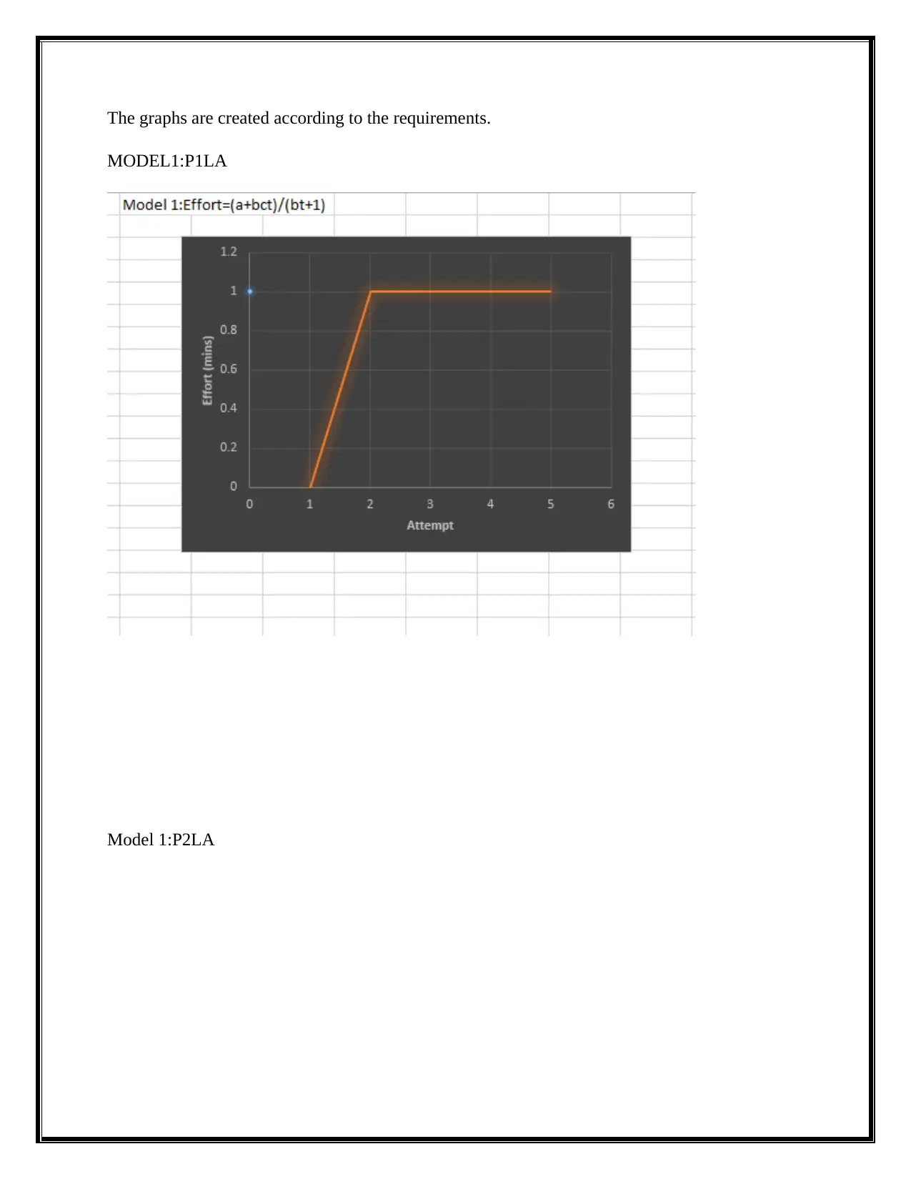
The graphs are created according to the requirements.
MODEL1:P1LA
Model 1:P2LA

Model 1:P1LB

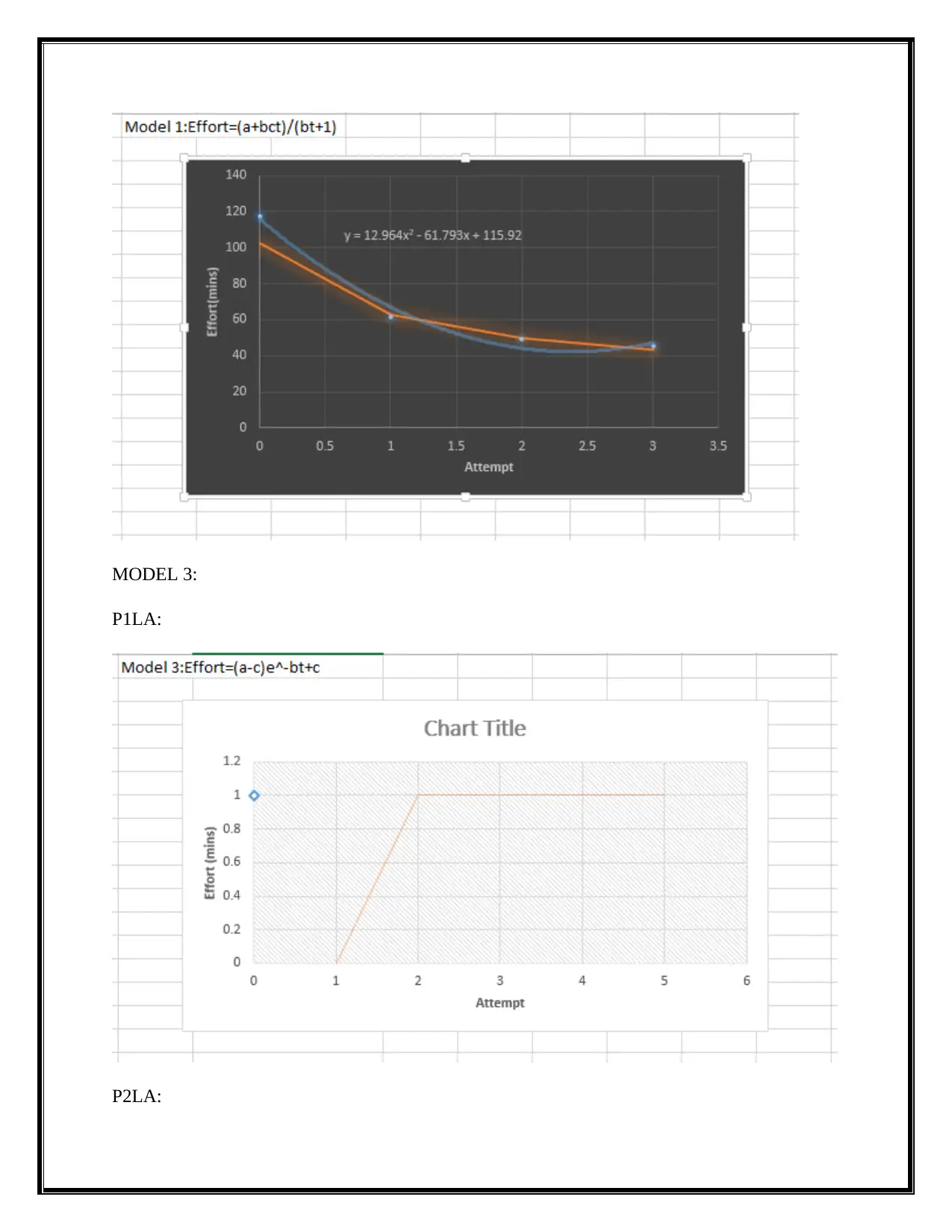
MODEL 3:
P1LA:
P2LA:

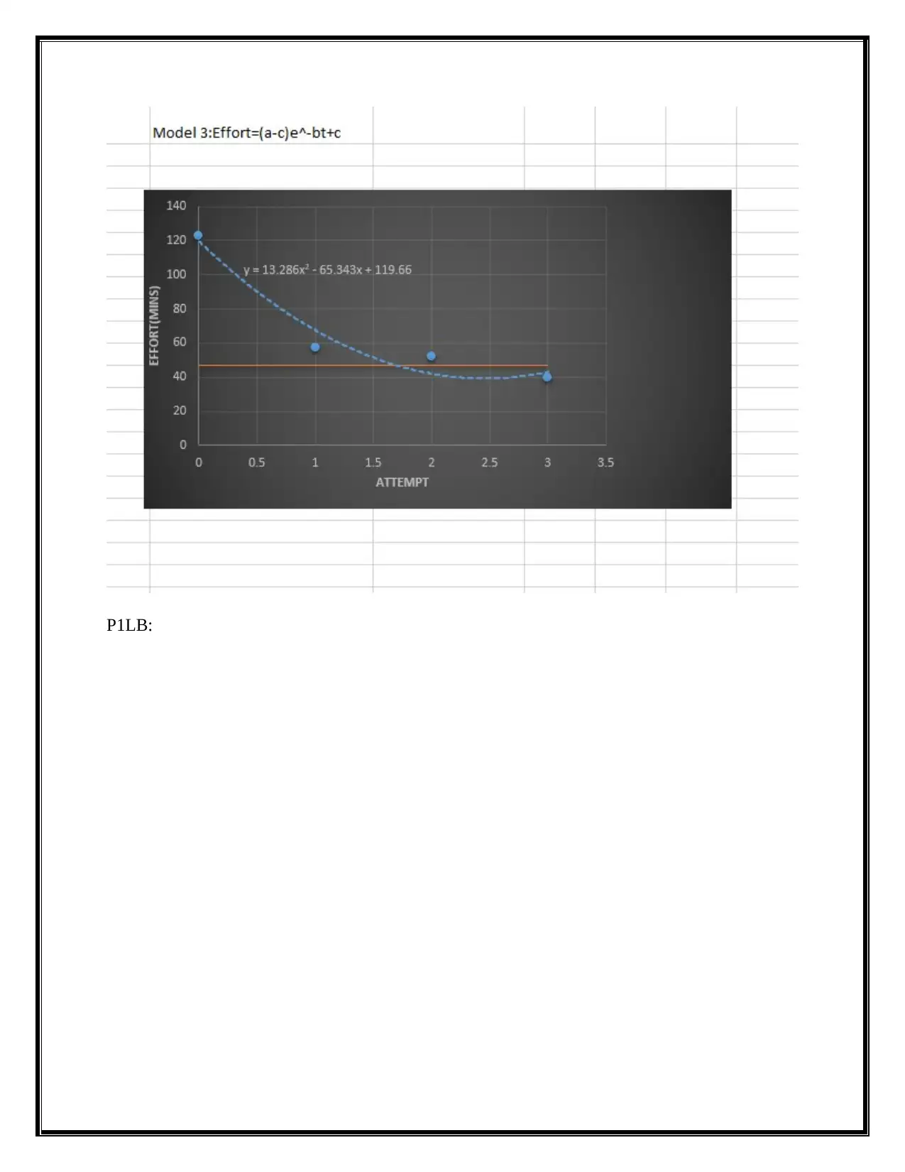
P1LB:

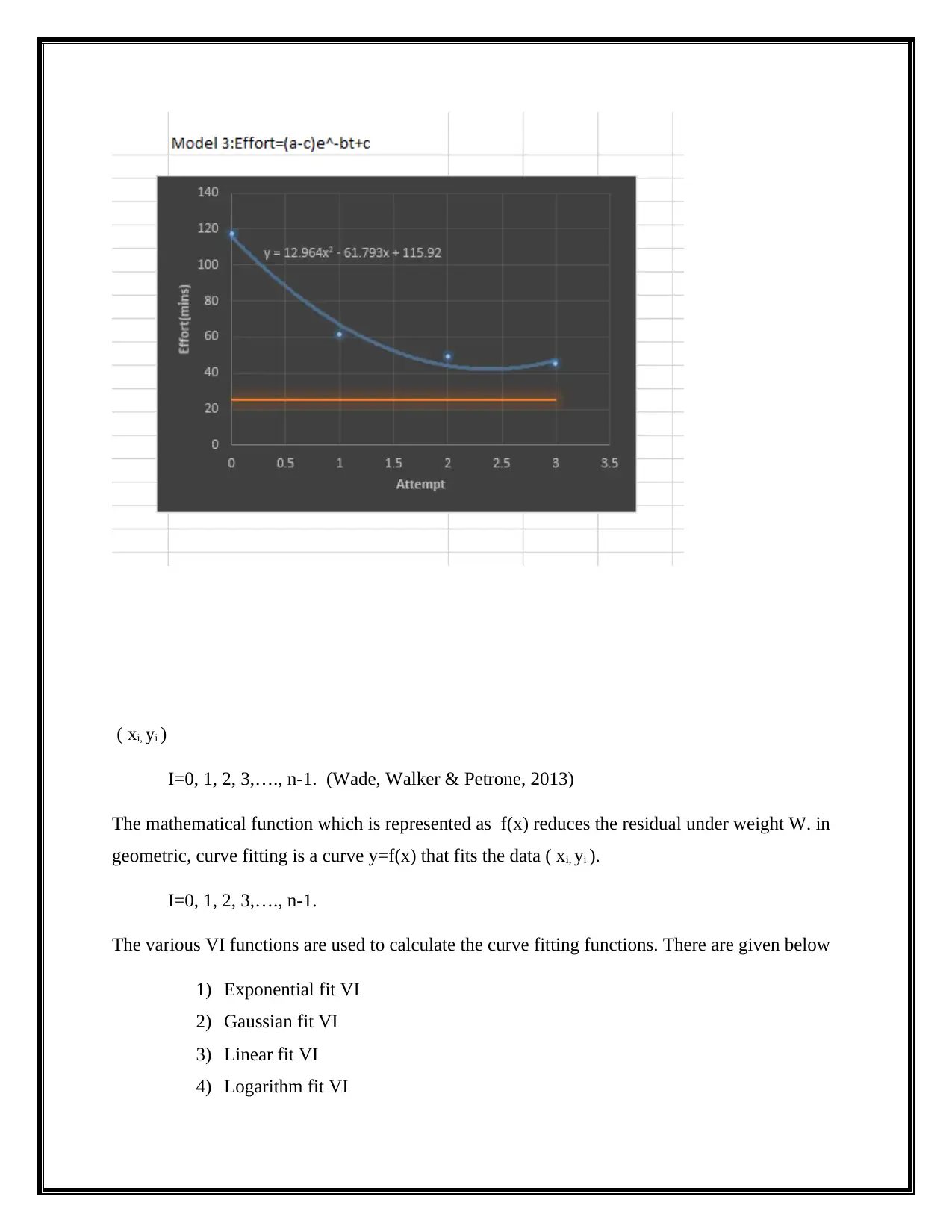
( xi, yi )
I=0, 1, 2, 3,…., n-1. (Wade, Walker & Petrone, 2013)
The mathematical function which is represented as f(x) reduces the residual under weight W. in
geometric, curve fitting is a curve y=f(x) that fits the data ( xi, yi ).
I=0, 1, 2, 3,…., n-1.
The various VI functions are used to calculate the curve fitting functions. There are given below
1) Exponential fit VI
2) Gaussian fit VI
3) Linear fit VI
4) Logarithm fit VI