Building & Evaluating Predictive Models: Data Analysis Report

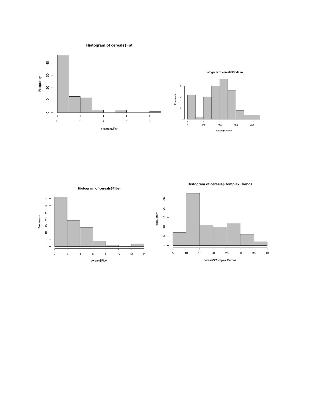
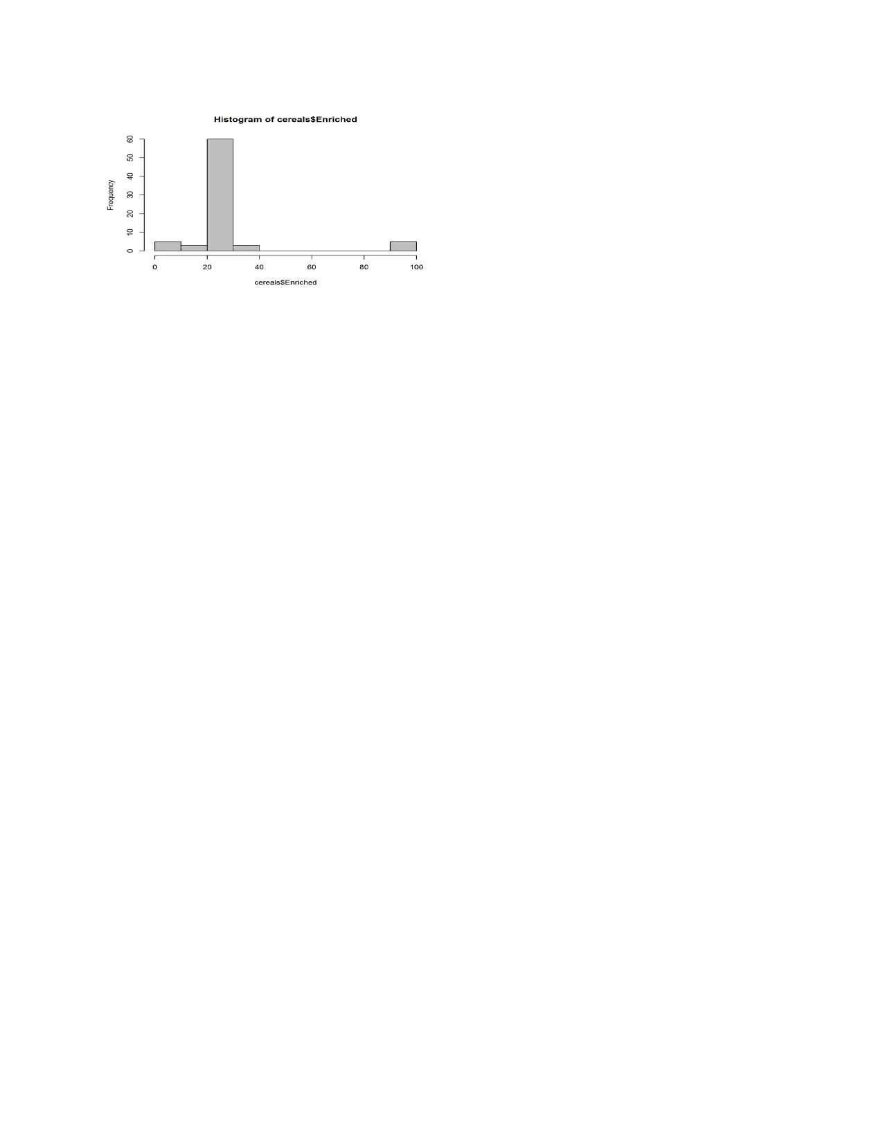
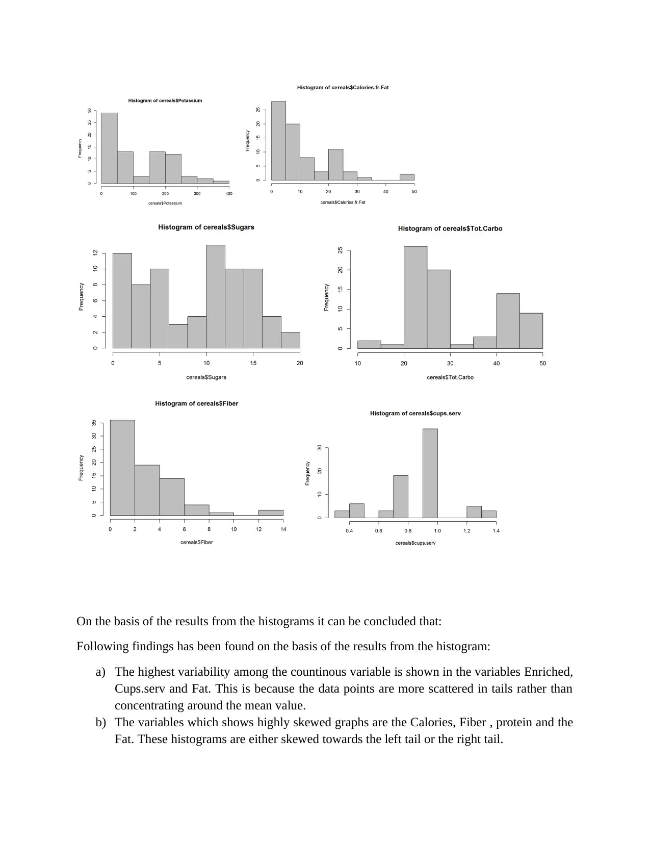
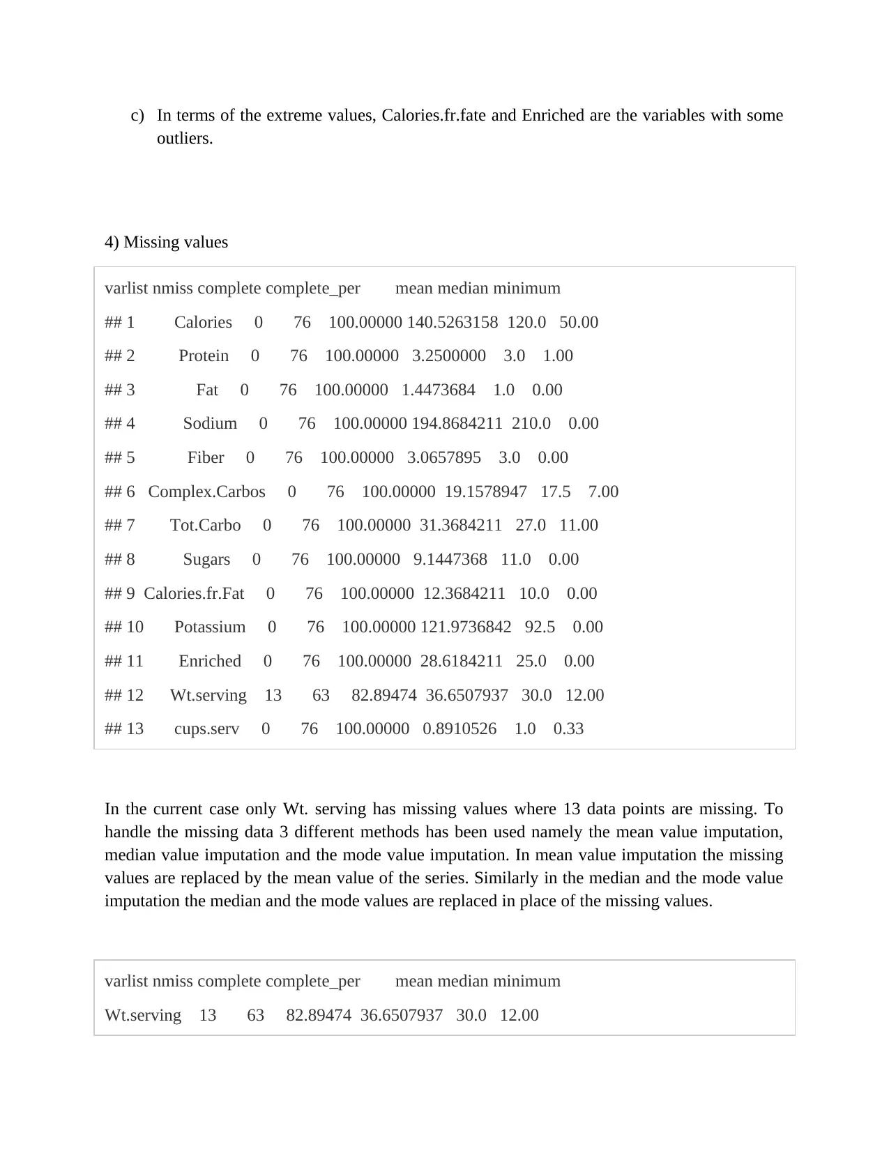
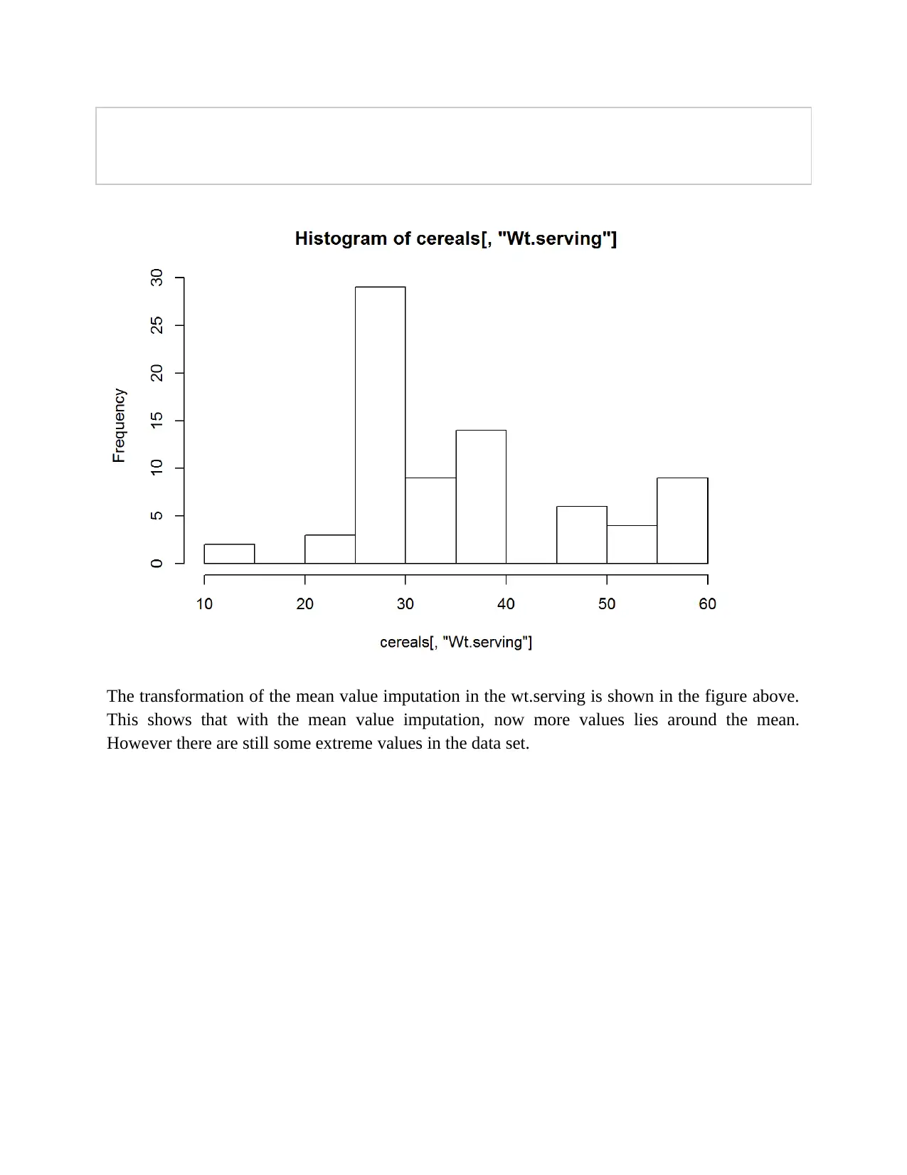
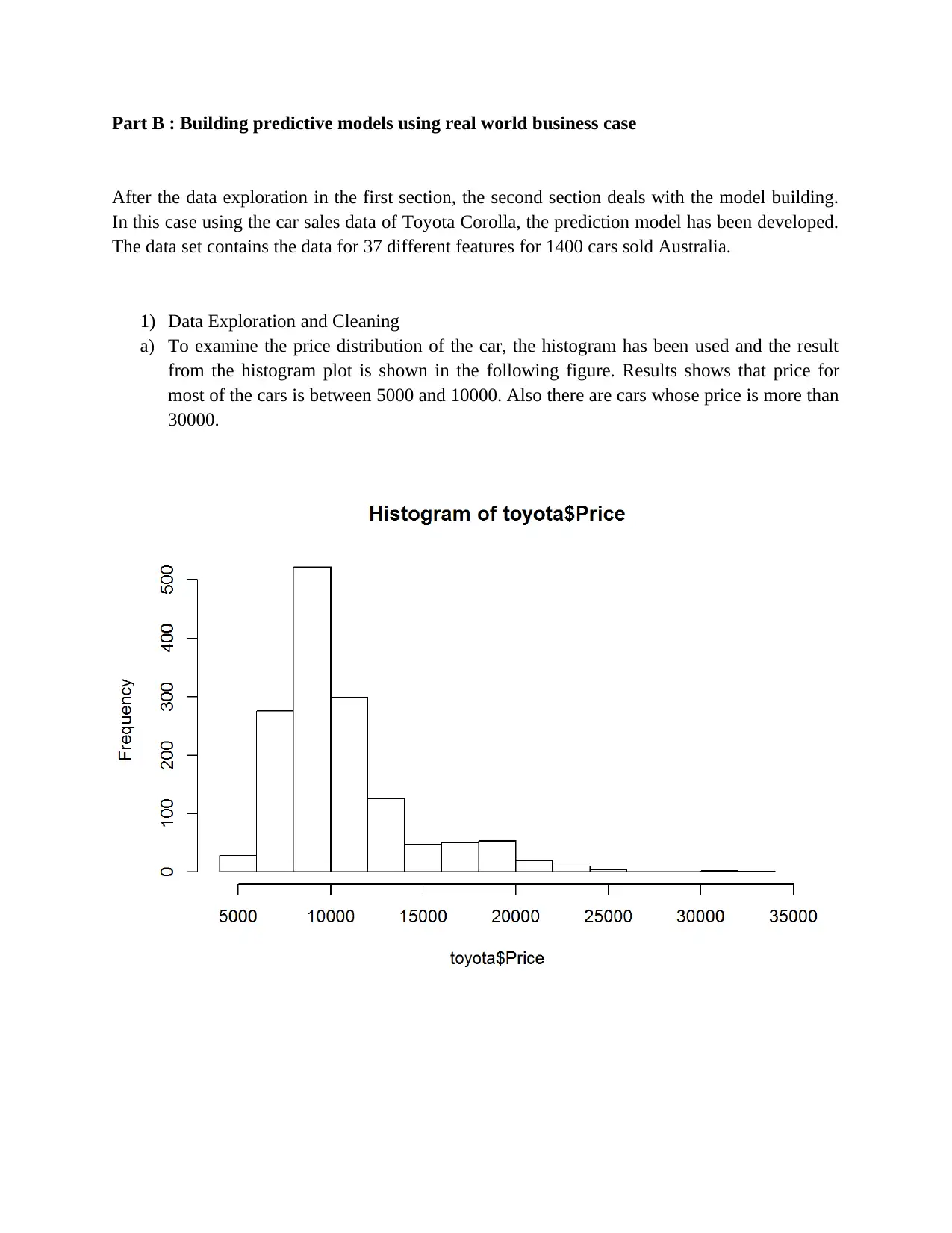
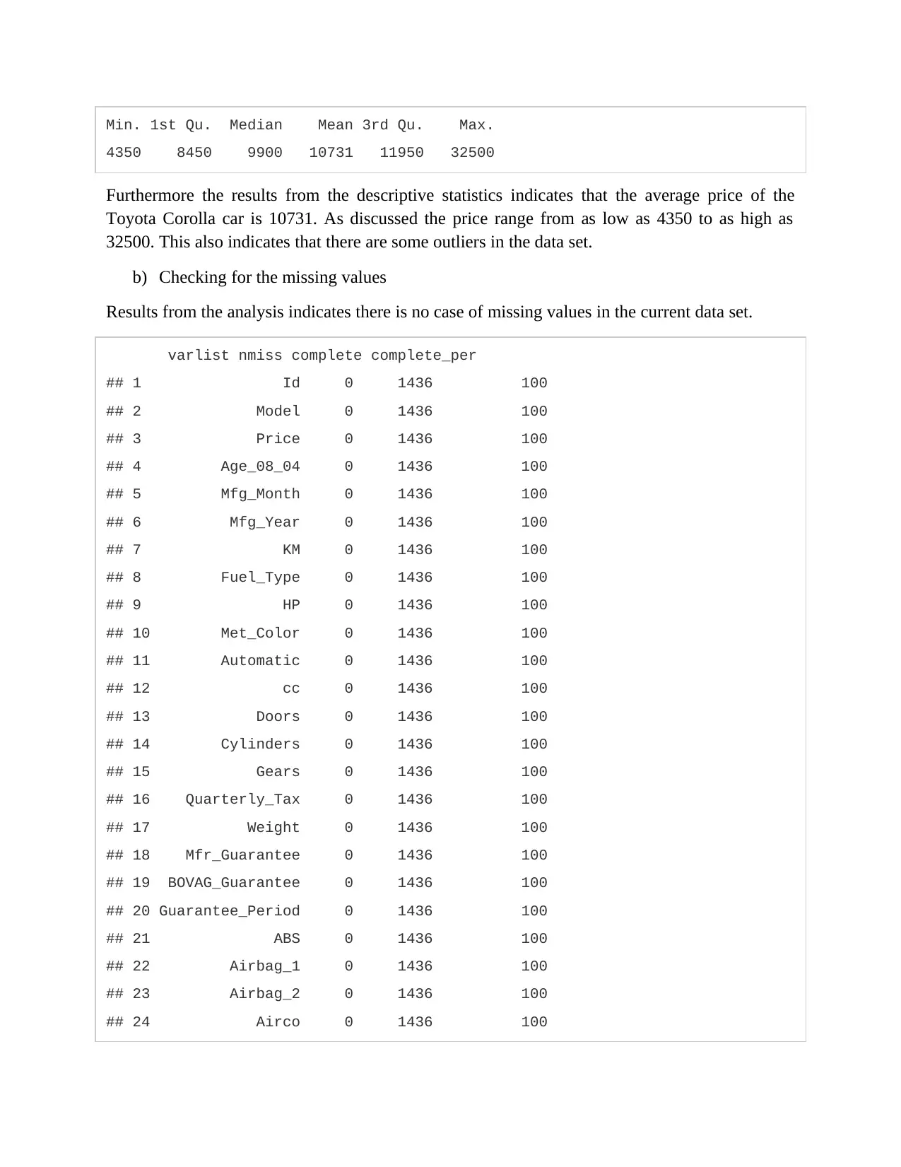
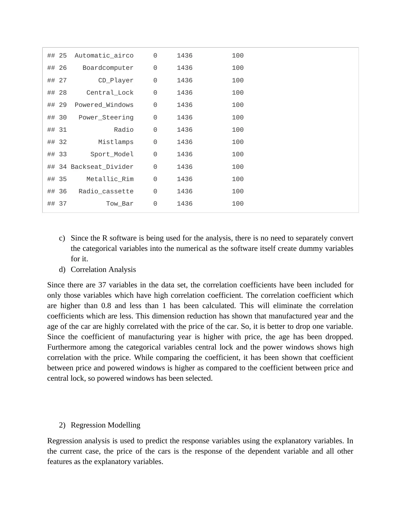
This assignment focuses on building and evaluating predictive models using two datasets: a cereal dataset for initial data exploration and cleaning, and a Toyota Corolla car sales dataset for regression modeling. The initial data exploration involves identifying continuous and categorical variables, calculating summary statistics, creating histograms to assess data distribution and skewness, and handling missing values using mean, median, and mode imputation. The second part involves building predictive models using the Toyota Corolla dataset. This includes examining price distribution, checking for missing values, performing correlation analysis to reduce dimensionality, and developing regression models to predict car prices. Several models are built, and iteratively improved based on the significance of coefficients and R-squared values, ultimately identifying an optimal model with highly significant coefficients.

Building and Evaluating Predictive Models
Part A: DATA EXPLORATION AND CLEANING
The first part of the research is focused on the data exploration and the cleaning of the given
data. For this part the cereals (for breakfast) data has been used. This data set contains 76 data
points and 18 different features. The results from the data exploration
1. The list of the continuous variables are shown in the table below.
## [1] "Calories" "Protein" "Fat"
## [4] "Sodium" "Fiber" "Complex.Carbos"
## [7] "Tot.Carbo" "Sugars" "Calories.fr.Fat"
## [10] "Potassium" "Enriched" "Wt.serving"
## [13] "cups.serv"
pTable 1 list of the numerical variables
Categorical variables are shown in the table below. The categorical variables are those variables
where there are more than one category. There are two types of the categorical variables. The
first one is the nominal variable where there is no particular order of the category. Secondly, the
other type of categorical variable is the ordinal variable, where the category have particular
order. In the current case among all the categorical variables, only Fibre.gr is the ordinal
variable. All other variables are the nominal variable.
# Ordinal: Fiber.Gr
# Nominal: Name, Manufacturer, Mfr, Hot.Cold
Table 2 Ordinal and the nominal variables

2. The summary statistics for the continuous variables has been calculated and for the
calculation purpose various measures of the central tendencies such as mean and median
has been included. The results are shown in the table below.
Calories Protein Fat Sodium
## C:73 Min. : 50.0 Min. :1.00 Min. :0.000 Min. : 0.0
## H: 3 1st Qu.:110.0 1st Qu.:2.00 1st Qu.:0.500 1st Qu.:147.5
## Median :120.0 Median :3.00 Median :1.000 Median :210.0
## Mean :140.5 Mean :3.25 Mean :1.447 Mean :194.9
## 3rd Qu.:192.5 3rd Qu.:5.00 3rd Qu.:2.000 3rd Qu.:262.5
## Max. :250.0 Max. :7.00 Max. :9.000 Max. :420.0
##
Fiber Complex.Carbos Tot.Carbo Sugars
## Min. : 0.000 Min. : 7.00 Min. :11.00 Min. : 0.000
## 1st Qu.: 1.000 1st Qu.:13.00 1st Qu.:24.00 1st Qu.: 4.000
## Median : 3.000 Median :17.50 Median :27.00 Median :11.000
## Mean : 3.066 Mean :19.16 Mean :31.37 Mean : 9.145
## 3rd Qu.: 5.000 3rd Qu.:26.00 3rd Qu.:41.00 3rd Qu.:14.000
## Max. :13.000 Max. :38.00 Max. :50.00 Max. :20.000
Calories.fr.Fat Potassium Enriched Wt.serving
## Min. : 0.00 Min. : 0.0 Min. : 0.00 Min. :12.00
## 1st Qu.: 5.00 1st Qu.: 35.0 1st Qu.: 25.00 1st Qu.:30.00
## Median :10.00 Median : 92.5 Median : 25.00 Median :30.00

## Mean :12.37 Mean :122.0 Mean : 28.62 Mean :36.65
## 3rd Qu.:20.00 3rd Qu.:200.0 3rd Qu.: 25.00 3rd Qu.:49.00
## Max. :50.00 Max. :390.0 Max. :100.00 Max. :60.00
## NA's :13
cups.serv Fiber.Gr
## Min. :0.3300 Low :33
## 1st Qu.:0.7500 Medium:32
## Median :1.0000 High :11
## Mean :0.8911
## 3rd Qu.:1.0000
## Max. :1.3300
Table 3 Table for the summary statistics
The summary statistics of the continuous variable is shown in the table above. On the basis of the
results, the variable which has extreme values is the potassium. In case of potassium the mean value is
194 whereas the minimum and the maxim value are 0 and 420 respectively. Similarly the range of
calories also lies between as low as 50 to as high as 250.
Count of the categorical variables
100% Bran : 1 American Home: 1 A: 1
## 100% Nat. Bran Oats & Honey : 1 General Mills:25 G:25
## 100% Nat. Low Fat Granola w raisins: 1 Kelloggs :23 K:23
## All-Bran : 1 Nabisco : 5 N: 5
## All-Bran with Extra Fiber : 1 Post :10 P:10
## Almond Crunch w Raisins : 1 Quaker Oats :12 Q:12
## (Other) :70

Fibre.Gr
# Low :33
## Medium:32
##High :11
In terms of the categorical variable, one of the variable hot and cold shows higher variation.
There are 73 cold cereals whereas the number of hot cereals is only 3.
Histogram of the variables (continuous) is shown below.

On the basis of the results from the histograms it can be concluded that:
Following findings has been found on the basis of the results from the histogram:
a) The highest variability among the countinous variable is shown in the variables Enriched,
Cups.serv and Fat. This is because the data points are more scattered in tails rather than
concentrating around the mean value.
b) The variables which shows highly skewed graphs are the Calories, Fiber , protein and the
Fat. These histograms are either skewed towards the left tail or the right tail.

c) In terms of the extreme values, Calories.fr.fate and Enriched are the variables with some
outliers.
4) Missing values
varlist nmiss complete complete_per mean median minimum
## 1 Calories 0 76 100.00000 140.5263158 120.0 50.00
## 2 Protein 0 76 100.00000 3.2500000 3.0 1.00
## 3 Fat 0 76 100.00000 1.4473684 1.0 0.00
## 4 Sodium 0 76 100.00000 194.8684211 210.0 0.00
## 5 Fiber 0 76 100.00000 3.0657895 3.0 0.00
## 6 Complex.Carbos 0 76 100.00000 19.1578947 17.5 7.00
## 7 Tot.Carbo 0 76 100.00000 31.3684211 27.0 11.00
## 8 Sugars 0 76 100.00000 9.1447368 11.0 0.00
## 9 Calories.fr.Fat 0 76 100.00000 12.3684211 10.0 0.00
## 10 Potassium 0 76 100.00000 121.9736842 92.5 0.00
## 11 Enriched 0 76 100.00000 28.6184211 25.0 0.00
## 12 Wt.serving 13 63 82.89474 36.6507937 30.0 12.00
## 13 cups.serv 0 76 100.00000 0.8910526 1.0 0.33
In the current case only Wt. serving has missing values where 13 data points are missing. To
handle the missing data 3 different methods has been used namely the mean value imputation,
median value imputation and the mode value imputation. In mean value imputation the missing
values are replaced by the mean value of the series. Similarly in the median and the mode value
imputation the median and the mode values are replaced in place of the missing values.
varlist nmiss complete complete_per mean median minimum
Wt.serving 13 63 82.89474 36.6507937 30.0 12.00

The transformation of the mean value imputation in the wt.serving is shown in the figure above.
This shows that with the mean value imputation, now more values lies around the mean.
However there are still some extreme values in the data set.

Part B : Building predictive models using real world business case
After the data exploration in the first section, the second section deals with the model building.
In this case using the car sales data of Toyota Corolla, the prediction model has been developed.
The data set contains the data for 37 different features for 1400 cars sold Australia.
1) Data Exploration and Cleaning
a) To examine the price distribution of the car, the histogram has been used and the result
from the histogram plot is shown in the following figure. Results shows that price for
most of the cars is between 5000 and 10000. Also there are cars whose price is more than
30000.

Min. 1st Qu. Median Mean 3rd Qu. Max.
4350 8450 9900 10731 11950 32500
Furthermore the results from the descriptive statistics indicates that the average price of the
Toyota Corolla car is 10731. As discussed the price range from as low as 4350 to as high as
32500. This also indicates that there are some outliers in the data set.
b) Checking for the missing values
Results from the analysis indicates there is no case of missing values in the current data set.
varlist nmiss complete complete_per
## 1 Id 0 1436 100
## 2 Model 0 1436 100
## 3 Price 0 1436 100
## 4 Age_08_04 0 1436 100
## 5 Mfg_Month 0 1436 100
## 6 Mfg_Year 0 1436 100
## 7 KM 0 1436 100
## 8 Fuel_Type 0 1436 100
## 9 HP 0 1436 100
## 10 Met_Color 0 1436 100
## 11 Automatic 0 1436 100
## 12 cc 0 1436 100
## 13 Doors 0 1436 100
## 14 Cylinders 0 1436 100
## 15 Gears 0 1436 100
## 16 Quarterly_Tax 0 1436 100
## 17 Weight 0 1436 100
## 18 Mfr_Guarantee 0 1436 100
## 19 BOVAG_Guarantee 0 1436 100
## 20 Guarantee_Period 0 1436 100
## 21 ABS 0 1436 100
## 22 Airbag_1 0 1436 100
## 23 Airbag_2 0 1436 100
## 24 Airco 0 1436 100

## 25 Automatic_airco 0 1436 100
## 26 Boardcomputer 0 1436 100
## 27 CD_Player 0 1436 100
## 28 Central_Lock 0 1436 100
## 29 Powered_Windows 0 1436 100
## 30 Power_Steering 0 1436 100
## 31 Radio 0 1436 100
## 32 Mistlamps 0 1436 100
## 33 Sport_Model 0 1436 100
## 34 Backseat_Divider 0 1436 100
## 35 Metallic_Rim 0 1436 100
## 36 Radio_cassette 0 1436 100
## 37 Tow_Bar 0 1436 100
c) Since the R software is being used for the analysis, there is no need to separately convert
the categorical variables into the numerical as the software itself create dummy variables
for it.
d) Correlation Analysis
Since there are 37 variables in the data set, the correlation coefficients have been included for
only those variables which have high correlation coefficient. The correlation coefficient which
are higher than 0.8 and less than 1 has been calculated. This will eliminate the correlation
coefficients which are less. This dimension reduction has shown that manufactured year and the
age of the car are highly correlated with the price of the car. So, it is better to drop one variable.
Since the coefficient of manufacturing year is higher with price, the age has been dropped.
Furthermore among the categorical variables central lock and the power windows shows high
correlation with the price. While comparing the coefficient, it has been shown that coefficient
between price and powered windows is higher as compared to the coefficient between price and
central lock, so powered windows has been selected.
2) Regression Modelling
Regression analysis is used to predict the response variables using the explanatory variables. In
the current case, the price of the cars is the response of the dependent variable and all other
features as the explanatory variables.