Multiple Regression Analysis: Predictive Analysis of Wagner Printers

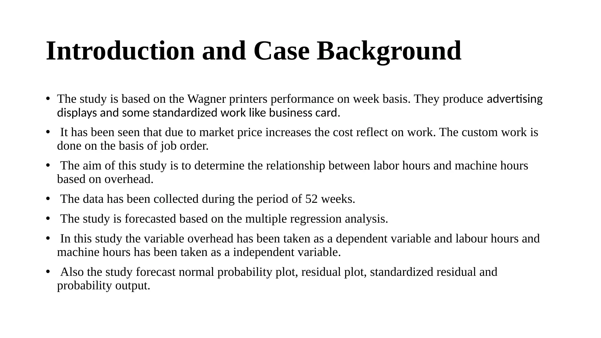
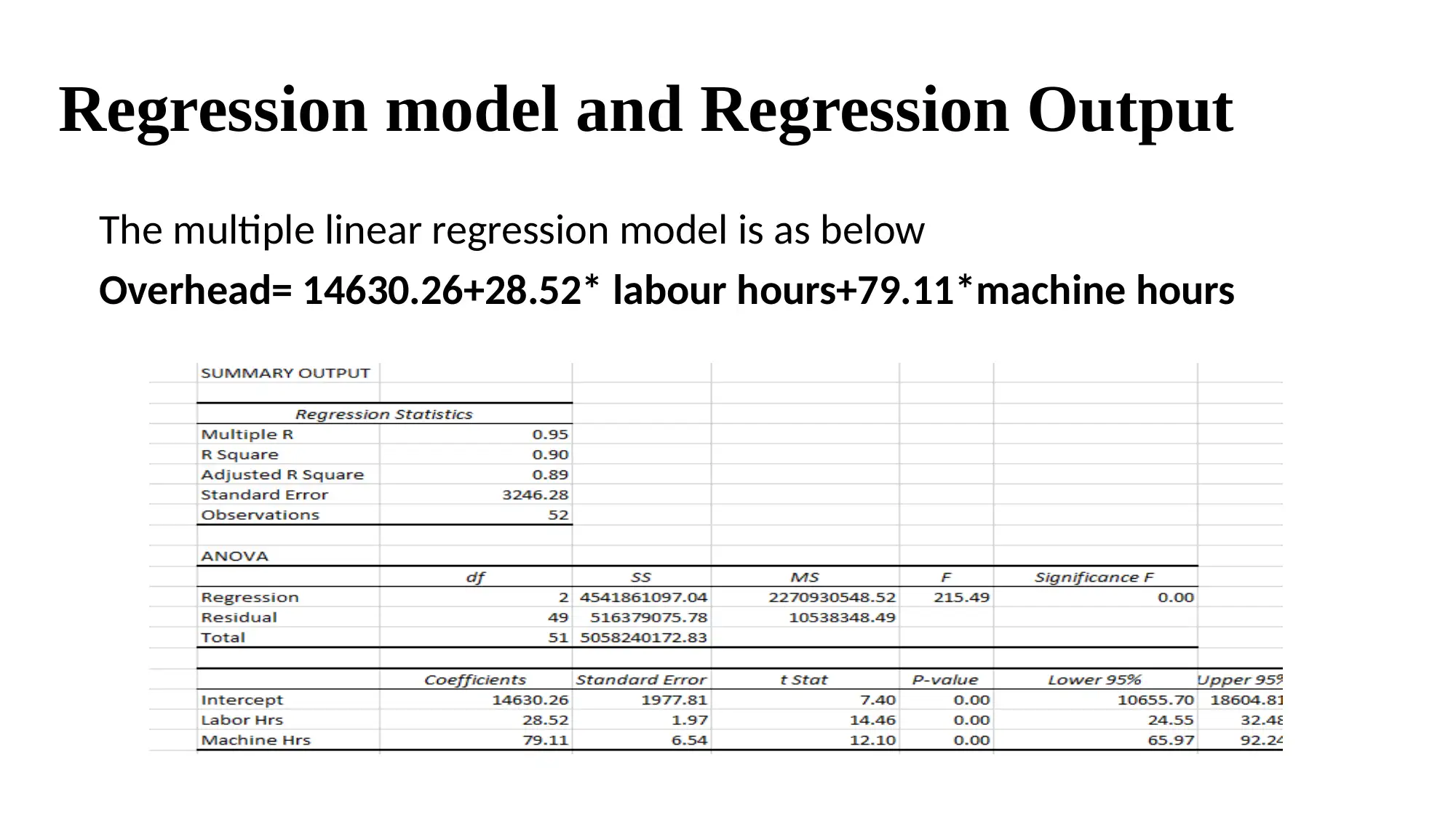
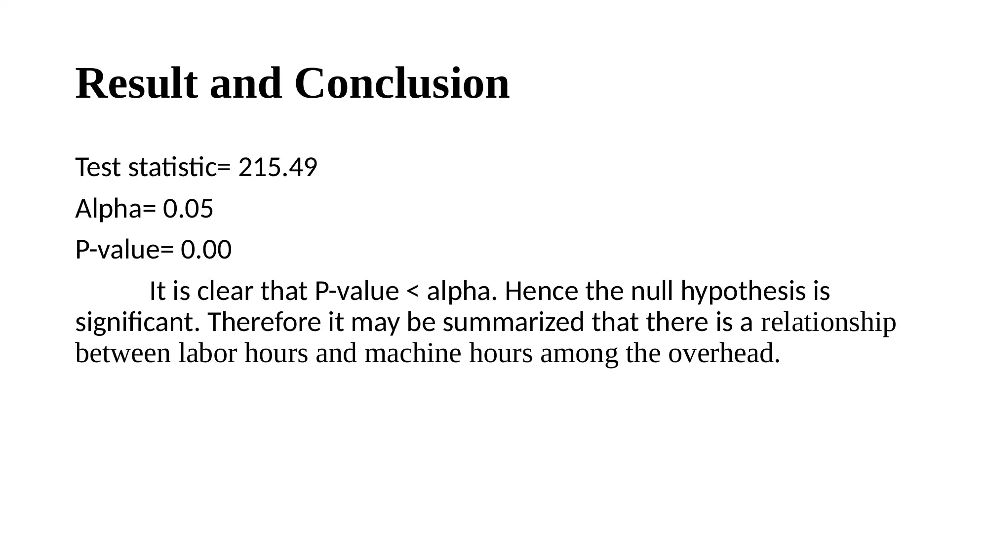
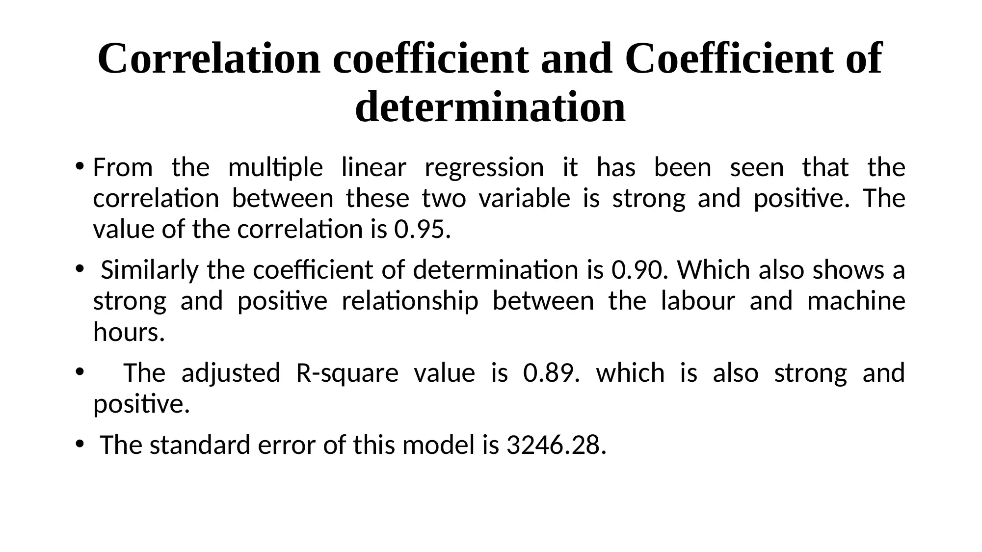
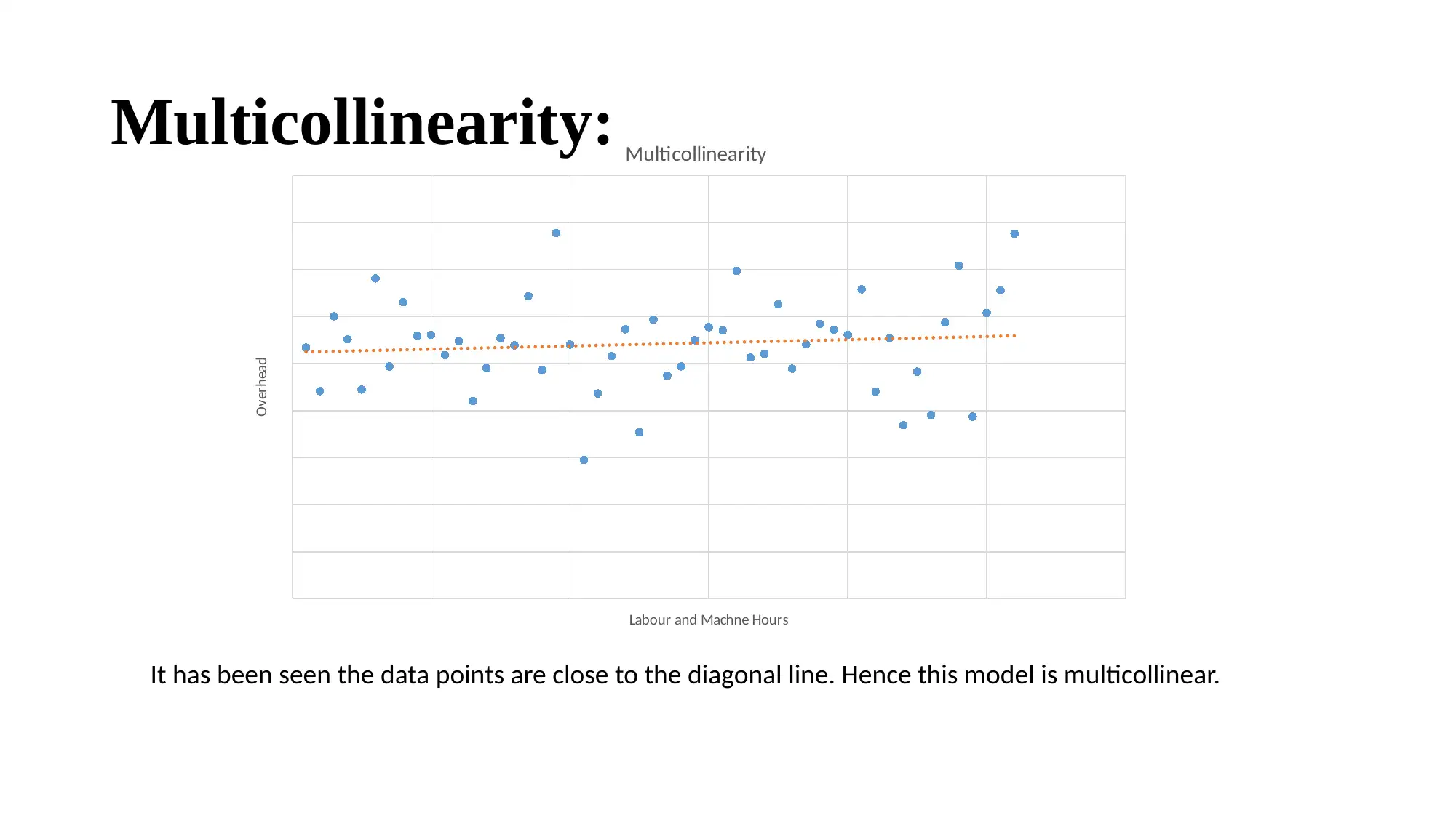
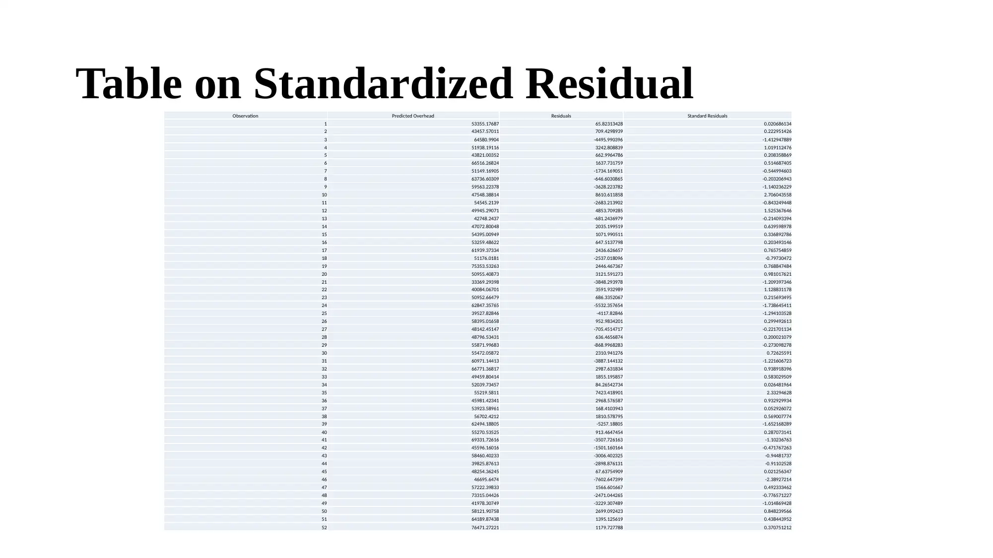
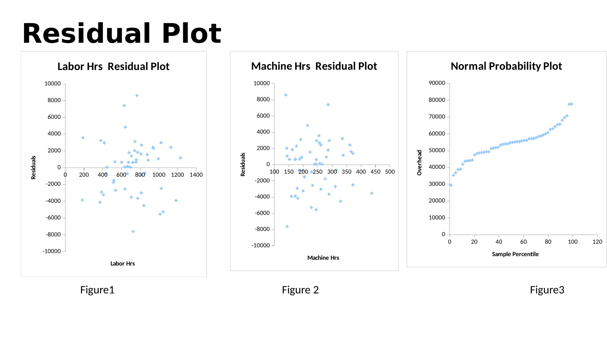
This report presents a predictive analysis of Wagner Printers' performance, focusing on the relationship between labor hours, machine hours, and overhead costs. The study utilizes multiple regression analysis to forecast overhead based on data collected over 52 weeks. The report includes a regression model, statistical outputs such as p-values and correlation coefficients, and hypothesis testing results. The analysis reveals a significant relationship between labor and machine hours and overhead, with a strong positive correlation and a high coefficient of determination. The report also addresses multicollinearity and assesses the model's residuals and normality. The conclusion highlights the effectiveness of regression analysis in predicting market and business trends, offering valuable insights into Wagner Printers' operational efficiency and cost management.

PREDICTIVE
ANALYSIS

Introduction and Case Background
• The study is based on the Wagner printers performance on week basis. They produce advertising
displays and some standardized work like business card.
• It has been seen that due to market price increases the cost reflect on work. The custom work is
done on the basis of job order.
• The aim of this study is to determine the relationship between labor hours and machine hours
based on overhead.
• The data has been collected during the period of 52 weeks.
• The study is forecasted based on the multiple regression analysis.
• In this study the variable overhead has been taken as a dependent variable and labour hours and
machine hours has been taken as a independent variable.
• Also the study forecast normal probability plot, residual plot, standardized residual and
probability output.

Hypothesis
Null hypothesis: There is no relationship between labor hours and
machine hours among the overhead.
Alternative hypothesis: There is a relationship between labor hours and
machine hours among the overhead.

Regression model and Regression Output
The multiple linear regression model is as below
Overhead= 14630.26+28.52* labour hours+79.11*machine hours

Result and Conclusion
Test statistic= 215.49
Alpha= 0.05
P-value= 0.00
It is clear that P-value < alpha. Hence the null hypothesis is
significant. Therefore it may be summarized that there is a relationship
between labor hours and machine hours among the overhead.

Correlation coefficient and Coefficient of
determination
• From the multiple linear regression it has been seen that the
correlation between these two variable is strong and positive. The
value of the correlation is 0.95.
• Similarly the coefficient of determination is 0.90. Which also shows a
strong and positive relationship between the labour and machine
hours.
• The adjusted R-square value is 0.89. which is also strong and
positive.
• The standard error of this model is 3246.28.

Multicollinearity: Multicollinearity
Labour and Machne Hours
Overhead
It has been seen the data points are close to the diagonal line. Hence this model is multicollinear.

Table on Standardized ResidualObservation Predicted Overhead Residuals Standard Residuals
1 53355.17687 65.82313428 0.020686134
2 43457.57011 709.4298939 0.222951426
3 64580.9904 -4495.990396 -1.412947889
4 51938.19116 3242.808839 1.019112476
5 43821.00352 662.9964786 0.208358869
6 66516.26824 1637.731759 0.514687405
7 51149.16905 -1734.169051 -0.544994603
8 63736.60309 -646.6030865 -0.203206943
9 59563.22378 -3628.223782 -1.140236229
10 47548.38814 8610.611858 2.706043558
11 54545.2139 -2683.213902 -0.843249448
12 49945.29071 4853.709285 1.525367646
13 42748.2437 -681.2436979 -0.214093394
14 47072.80048 2035.199519 0.639598978
15 54395.00949 1071.990511 0.336892786
16 53259.48622 647.5137798 0.203493146
17 61939.37334 2436.626657 0.765754859
18 51176.0181 -2537.018096 -0.79730472
19 75353.53263 2446.467367 0.768847484
20 50955.40873 3121.591273 0.981017621
21 33369.29398 -3848.293978 -1.209397346
22 40084.06701 3591.932989 1.128831178
23 50952.66479 686.3352067 0.215693495
24 62847.35765 -5532.357654 -1.738645411
25 39527.82846 -4117.82846 -1.294103528
26 58395.01658 952.9834201 0.299492613
27 48142.45147 -705.4514717 -0.221701134
28 48796.53431 636.4656874 0.200021079
29 55871.99683 -868.9968283 -0.273098278
30 55472.05872 2310.941276 0.72625591
31 60971.14413 -3887.144132 -1.221606723
32 66771.36817 2987.631834 0.938918396
33 49459.80414 1855.195857 0.583029509
34 52039.73457 84.26542734 0.026481964
35 55219.5811 7423.418901 2.33294628
36 45981.42341 2968.576587 0.932929934
37 53923.58961 168.4103943 0.052926072
38 56702.4212 1810.578795 0.569007774
39 62494.18805 -5257.18805 -1.652168289
40 55270.53525 913.4647454 0.287073141
41 69331.72616 -3507.726163 -1.10236763
42 45596.16016 -1501.160164 -0.471767263
43 58460.40233 -3006.402325 -0.94481737
44 39825.87613 -2898.876131 -0.91102528
45 48254.36245 67.63754909 0.021256347
46 46695.6474 -7602.647399 -2.38927214
47 57222.39833 1566.601667 0.492333462
48 73315.04426 -2471.044265 -0.776571227
49 41978.30749 -3229.307489 -1.014869428
50 58121.90758 2699.092423 0.848239566
51 64189.87438 1395.125619 0.438443952
52 76471.27221 1179.727788 0.370751212

Residual Plot
0 200 400 600 800 1000 1200 1400
-10000
-8000
-6000
-4000
-2000
0
2000
4000
6000
8000
10000
Labor Hrs Residual Plot
Labor Hrs
Residuals
100 150 200 250 300 350 400 450 500
-10000
-8000
-6000
-4000
-2000
0
2000
4000
6000
8000
10000
Machine Hrs Residual Plot
Machine Hrs
Residuals
0 20 40 60 80 100 120
0
10000
20000
30000
40000
50000
60000
70000
80000
90000
Normal Probability Plot
Sample Percentile
Overhead
Figure1 Figure 2 Figure3

Conclusion
• From figure 1 and 2 there are some residuals has been seen.
• There some standardized residual is positive and some of negative.
• In figure 2 between 100 and 200 the highest residual has been seen
and the in the figure 1, between 500 and 1000 the maximum residual
is defined.
• The normal probability plot shows that the model is normal among
the variable.
• Yes, the regression analysis is a good method in prediction and data
analysis, which is easily predict the future of market and business.

THANK YOU