Financial Econometrics: Pricing Factor Models and Diagnostic Tests

This assignment analyzes financial pricing factors based on the Fama and French (1996) model, focusing on market risk premium, high minus low (value premium), and small minus big factors. It involves computing these factors, providing descriptive statistics and graphs for SMALL_HiBM and BIG_LoBM portfolios, and interpreting their characteristics. The assignment further explores the expected signs of coefficients in the pricing equations and estimates the models, interpreting the fitted coefficients and assessing their statistical significance. The solution then tests the validity of the CAPM relative to the three-factor model and conducts diagnostic tests, including auto-collinearity, heteroskedasticity, and non-normality, to assess the reliability of the estimated models. Finally, the assignment discusses potential solutions to address any identified issues in the data analysis process.

1
Part A
Question 1
How are the pricing factors computed and what do they represent? (hint: read the Fama
and French (1996) paper – its on iLearn). Provide graphs and descriptive statistics for the
SMALL_HiBM and BIG_LoBM portfolios and comment on their main characteristics. (5
marks)
There are three main pricing factors these include the market risk premium, high minus low and
small minus big. There are specific methods of computing each of these three pricing factors.
Market risk premium
Market risk premium comprises of the variance between the predictable return and the risk-free
rate on the market portfolio. This market risk premium is the same as the incline of the security
market line. There are three major market concepts to consider in computing market risk
premium. These include required market risk premium, expected market risk premium and the
historical market risk premium. Calculating this risk premium involves: finding the difference
between the expected market premium and risk-free rate.
Market risk premium =Expected market return-Risk free rate.
Therefore, this price factor model is used by investors to measure their possibility that the
investments will yield adequate returns to the investors. The presence of risk factor is one of the
essential elements of a market that determines the rate of performance. A risk-free investment
does not demonstrate a high level of return hence it does not become significant to the operations
of the firms.

2
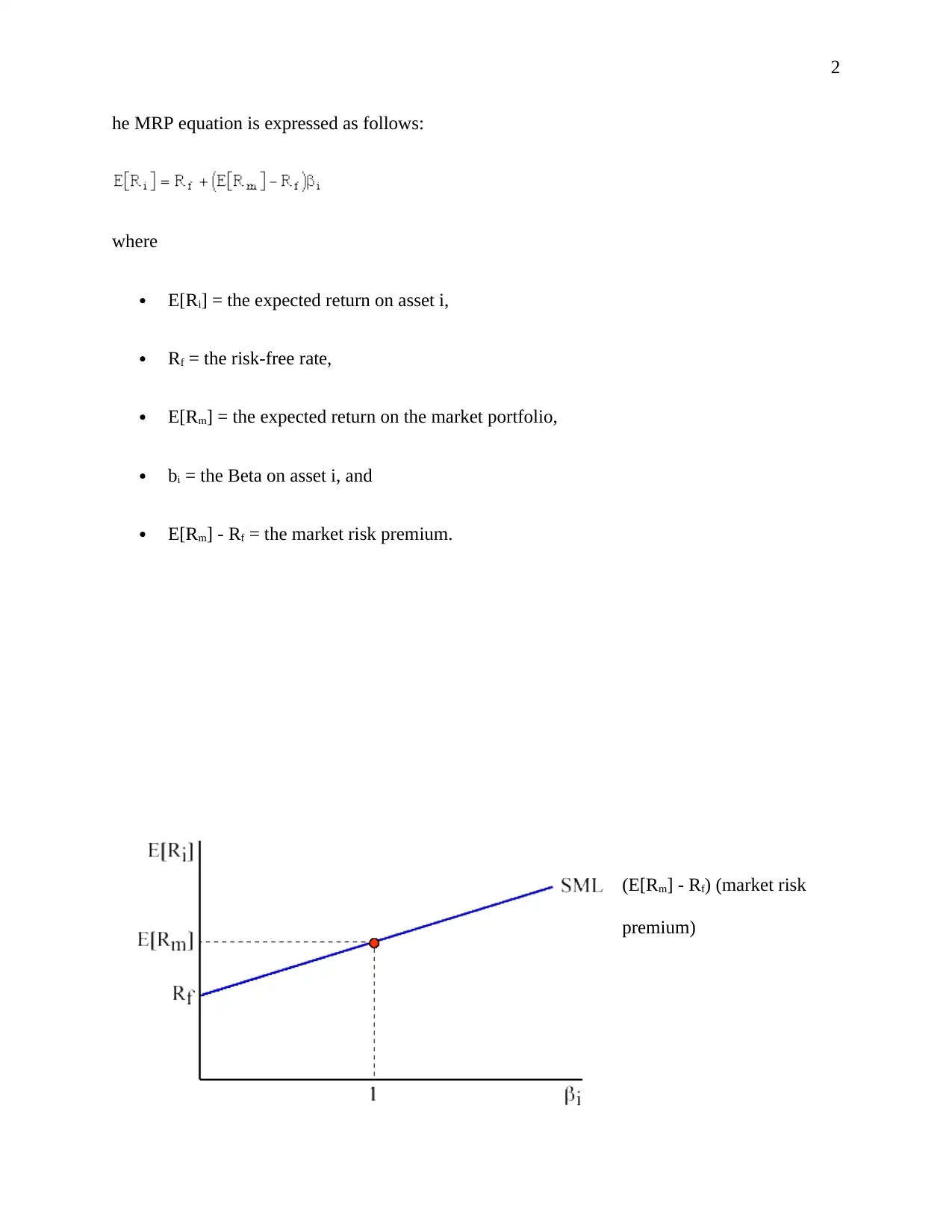
he MRP equation is expressed as follows:
where
 E[Ri] = the expected return on asset i,
 Rf = the risk-free rate,
 E[Rm] = the expected return on the market portfolio,
 bi = the Beta on asset i, and
 E[Rm] - Rf = the market risk premium.
(E[Rm] - Rf) (market risk
premium)

3
High minus Low
High minus Low is also termed as value premium. This strategy is always based on the book
value, and it has it states that a higher book value in the market stock are termed as a value stock,
while the lower book value of the market stock is termed as a growth stock. Therefore value
stock has a tendency to give higher returns than the growth stock. Growth stock, which is
associated with growing firms, may show an increased rates, but the actual performance is still
minimal as compared to the value stock
Calculation of high minus low therefore involve determining both the market value and the book
value of the stock
Market value = number id outstanding shares * current market price in the stock
= N * CMP
r - Rf = [ B3 * (Km - Rf) ] + [ Bs * SMB ] + [ Bv * HML ] + [A]
Here,
r = Portfolio’s return rate,
Rf = Risk-free return rate,
B3 = Three factor beta,
Km = Returns of the market,
Bs = ‘0’ to ’1’, based on the portfolio. ‘1’ for pure small cap portfolio and
Bv = ‘0’ to ’1’, based on the portfolio. ‘1’ for value stocks, ‘0’ for growth stocks.

4
Book value is determined by looking at the historical accounting and cost of the company. Use
the book value and the market value to find the HML. The ratio will determine whether a stock is
a value stock or a growth stock.
Small minus big
This model focuses on the speed of returns between small firms and the large-sized firms, and it
is based on the capitalization of the company's market. The principle behind this model is that
there is a tendency of small effect in small firms to outperform the same effects in the big firms.
Computation of small minus big involves:
SMB= 1/3(small value small neutral +small growth) - 1/3(big value+ big neutral +big growth)

5
Question 2
What signs (positive or negative) would you expect to estimate for each of the factors in
equations (1) and (2)? Explain the reasoning behind your answers? (5 marks)
Since there is always a great portfolio effect on small firms than the big firms, there is always a
tendency of such firms to reflect positive coefficients on various factored, since the firms are still
in growth stage, there is a probability that it will be affected by the most market factor in its
growth. Therefore, based on the regression analysis, the coefficient for Bo is likely to be
positive. Moreover, for each variable in the equation, there is the here is a likelihood that the
coefficients will reflect positivity throughout the equation.
Equation 2
This equation is a characteristic of a big company which has achieved a maturity level. For this
equation, there is a tendency of reduced effect in the various coefficients of the equation,
therefore, there is a likelihood that the factor coefficient relates negatively to the variables. This,
therefore, explains the reason why most coefficients of the variable are likely to be negative, The
negative relation indicates little effect of the variable on the market risk for a bigger company.
Question 3

6
. Estimate both models given in question 2, and present the fitted equations. Interpret the
fitted coefficients. Which parameters are statistically significant at the 5% level? Are the
estimated parameters of the same sign as what you expected in Question 2? (5 marks)
Estimate both models given in question 2, and present the fitted equations. Interpret the fitted
coefficients. Which parameters are statistically significant at the 5% level? Are the estimated
parameters of the same sign as what you expected in Question 2?
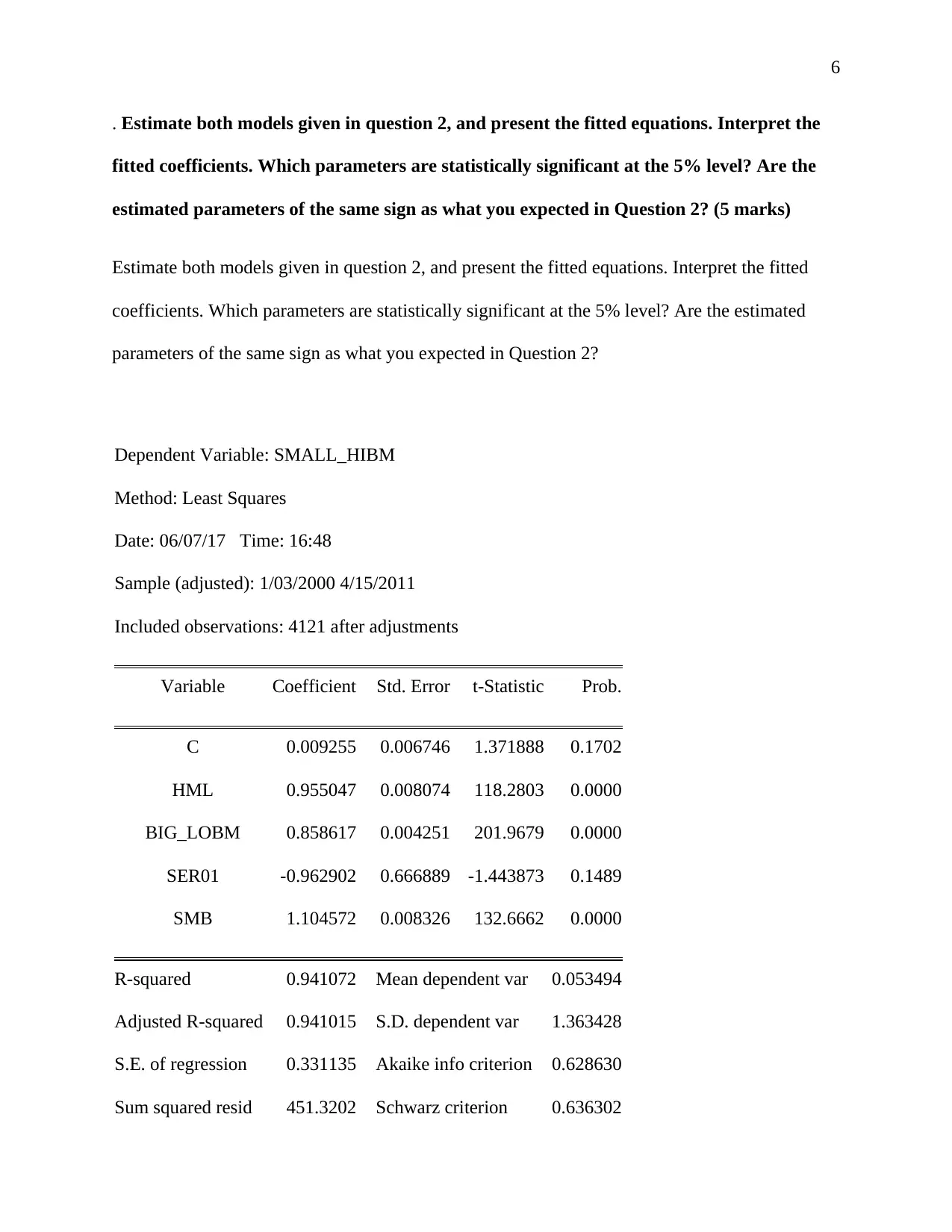
Dependent Variable: SMALL_HIBM
Method: Least Squares
Date: 06/07/17 Time: 16:48
Sample (adjusted): 1/03/2000 4/15/2011
Included observations: 4121 after adjustments
Variable Coefficient Std. Error t-Statistic Prob.
C 0.009255 0.006746 1.371888 0.1702
HML 0.955047 0.008074 118.2803 0.0000
BIG_LOBM 0.858617 0.004251 201.9679 0.0000
SER01 -0.962902 0.666889 -1.443873 0.1489
SMB 1.104572 0.008326 132.6662 0.0000
R-squared 0.941072 Mean dependent var 0.053494
Adjusted R-squared 0.941015 S.D. dependent var 1.363428
S.E. of regression 0.331135 Akaike info criterion 0.628630
Sum squared resid 451.3202 Schwarz criterion 0.636302

7
Log likelihood -1290.291 Hannan-Quinn criter. 0.631345
F-statistic 16432.93 Durbin-Watson stat 1.960122
Prob(F-statistic) 0.000000
Dependent Variable: BIG_LOBM
Method: Least Squares
Date: 06/07/17 Time: 17:07
Sample (adjusted): 1/03/2000 5/14/2011
Included observations: 4150 after adjustments
Variable Coefficient Std. Error t-Statistic Prob.
C
0.0121467
152261579
8
0.00302261
999968307
8
4.01860479
565131
5.958260
42428455
4e-05
HML
-
0.3174377
178438972
0.00467707
013496350
1
-
67.8710621
5724398 0
SMB
-
0.1776227
938788975
0.00493201
854771043
7
-
36.0142185
5182487
2.253819
43488334
9e-247

8
MKT_RF
0.9520223
100404066
0.00240397
967549622
3
396.019284
0831289 0
R-squared
0.9750760
237825671 Mean dependent var
0.021660
24096385
544
Adjusted R-squared
0.9750579
890675038 S.D. dependent var
1.231909
44568453
8
S.E. of regression
0.1945559
503051971 Akaike info criterion
-
0.435230
53308223
48
Sum squared resid
156.93446
57953104 Schwarz criterion
-
0.429128
49586466
88
Log likelihood
907.10335
61456372 Hannan-Quinn criter.
-
0.433071
56030948
91
F-statistic
54066.616
5427074 Durbin-Watson stat
1.991504
12188114

9
Prob(F-statistic) 0
Most of the coefficients anticipated were negative; therefore, it proves the prediction above.
BIG_LOBM=0.012147+0.95202- 0.317248-0.177623
This gives the numerical values for the above equations. The above equation, therefore,
represent a kind od of relationship that is characterized by negativity. , this is a sign of little
effect of the variable on the given market
Part B
Question 4
Conduct a test for the validity of the CAPM relative to the threefactor model. What
do you find
A test for the validity of the CAPM
CAPM reveals that Small minus big pricing has a positive value of 1.10 in the case of the small
firm. This reveals that there is a tendency by small firms to yield more, for a given change in the
market factor. The result of the analysis as indicated by the analysis above is a clear indication of
the factors. On the other hand, the value of SMB in the case of the big company had a value less
than one. This indicates a little benefit by the company
While focusing on the high-low pricing model, there is a tendency by small firms to record a
higher reading than the big firms. Therefore, it becomes clear that big firms have lower value

10
premium. In this case, the small firms are linked to growth stock, while big firms are associated
with value stock.
Question 5.
Conduct the basic diagnostic tests on both estimated models (equations (1) and (2))
a) auto colinearity
Based on the analysis for equation one in the data analysis above, the there was no relationship
between the various residuals of the variables this, therefore, indicated nonexistence of auto
colinearity in the data. On the other hand, the second equation also lacked auto colinearity since
the existence of the of non-related residuals in the data became a clear indication of the
nonexistence of auto colinearity. Therefore there rise of this defect that is attributed to the
existence if the relation between among the different independent variable lead to a misleading
interpretation of the various results obtained from the data set.
-12
-8
-4
0
4
8
12
00 01 02 03 04 05 06 07 08 09 10 11 12 13 14 15 16
HML MKT_RF

11
B) Heteroskedasticity (no cross product)
In equation one, according to the analysis, there was no direct relationship between the
independent variables. This is an indication of non-presence of heteroscedasticity. On the other
hand, this concept also applies to the second equation where the presence of heteroscedasticity
was tested, therefore, the non-existence of the heteroscedasticity in both the data revealed
perfection of the various in the data. Heterscedas
Heteroskedasticity Test: Breusch-Pagan-Godfrey
F-statistic
21.21941253
28928 Prob. F(4,4145)
2.42382403
0636759e-
17
Obs*R-squared
83.27480773
23383 Prob. Chi-Square(4) 0
Scaled explained SS
245.4710027
846494 Prob. Chi-Square(4) 0
d) Non-normality
There was an absence of not- normality of the data since the presence of consistency in the R-
squares was logical and presentable. The non-normally for the data used in the analysis,
therefore, can be determined through testing for the existence of the extreme vales in the data set.
This leads to exaggerated results that do not reflect the true result of the f phenomenon. In the
case of the data set for our analysis, there was no any element of non-normalcy

12
0
200
400
600
800
1,000
-1.5 -1.0 -0.5 0.0 0.5 1.0
Series: Residuals
Sample 1/03/2000 6/30/2016
Observations 4150
Mean -3.35e-17
Median -0.001312
Maximum 1.165802
Minimum -1.516103
Std. Dev. 0.194261
Skewness 0.001523
Kurtosis 6.909676
Jarque-Bera 2643.131
Probability 0.000000
d) Misspecification of functional form
There was some existence of miss-specification of the functions. The misplacement of the data
could be seen in the various dataset. The misspecification, therefore, could lead to wrong
information conclusion about the time series data and that the tendency to change information
miss specify the data set and lead to misleading R-squares in the analysis. This happens during
the data collection and recording, especially those that involve panel data.
Breusch-Godfrey Serial Correlation LM Test:
F-statistic
0.477655737
3892707 Prob. F(1,4144)
0.48952480
67881056
Obs*R-squared
0.478292193
8116025 Prob. Chi-Square(1)
0.48919690
26509349