University of Tasmania BEA121: Principles of Economics 2 Assignment

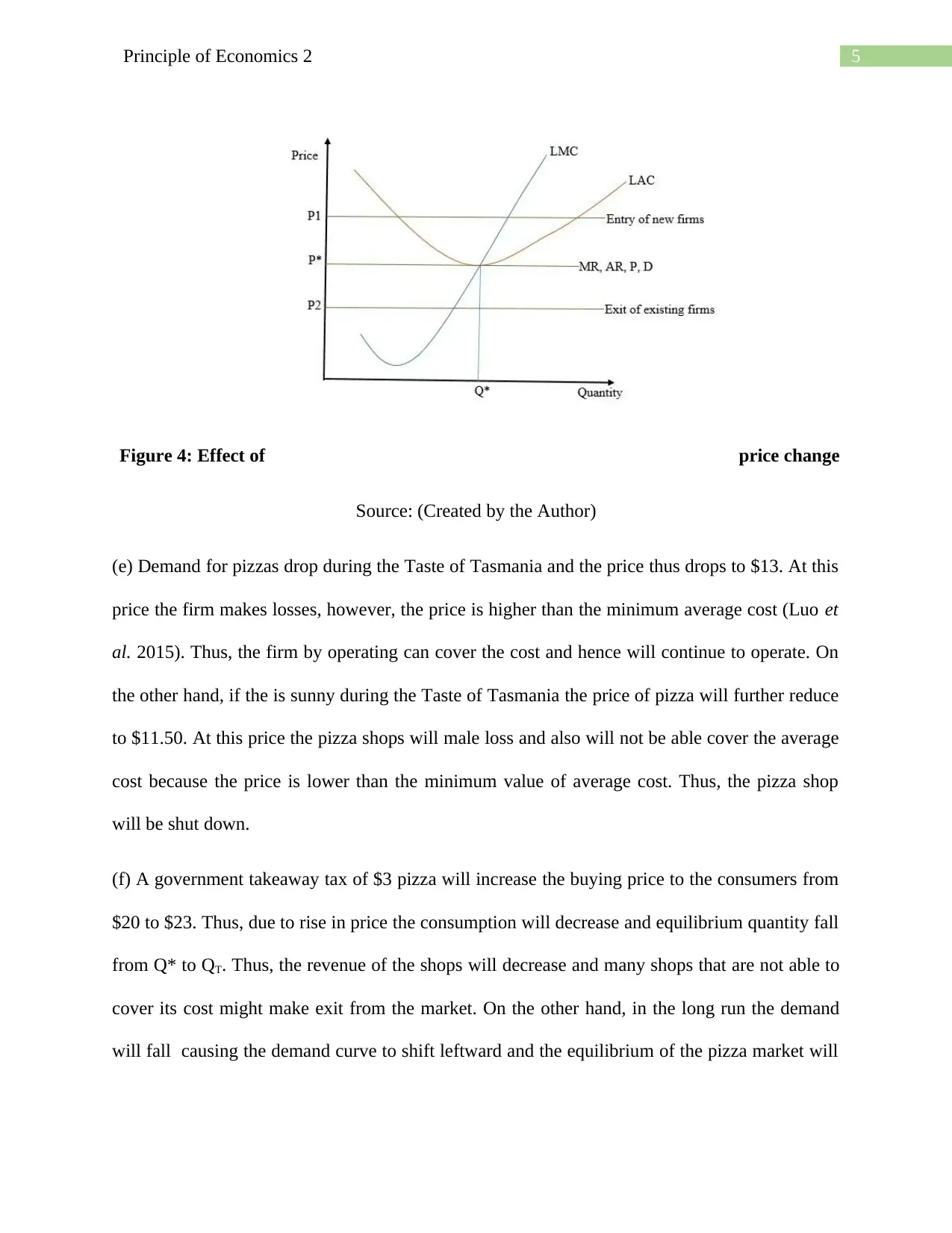
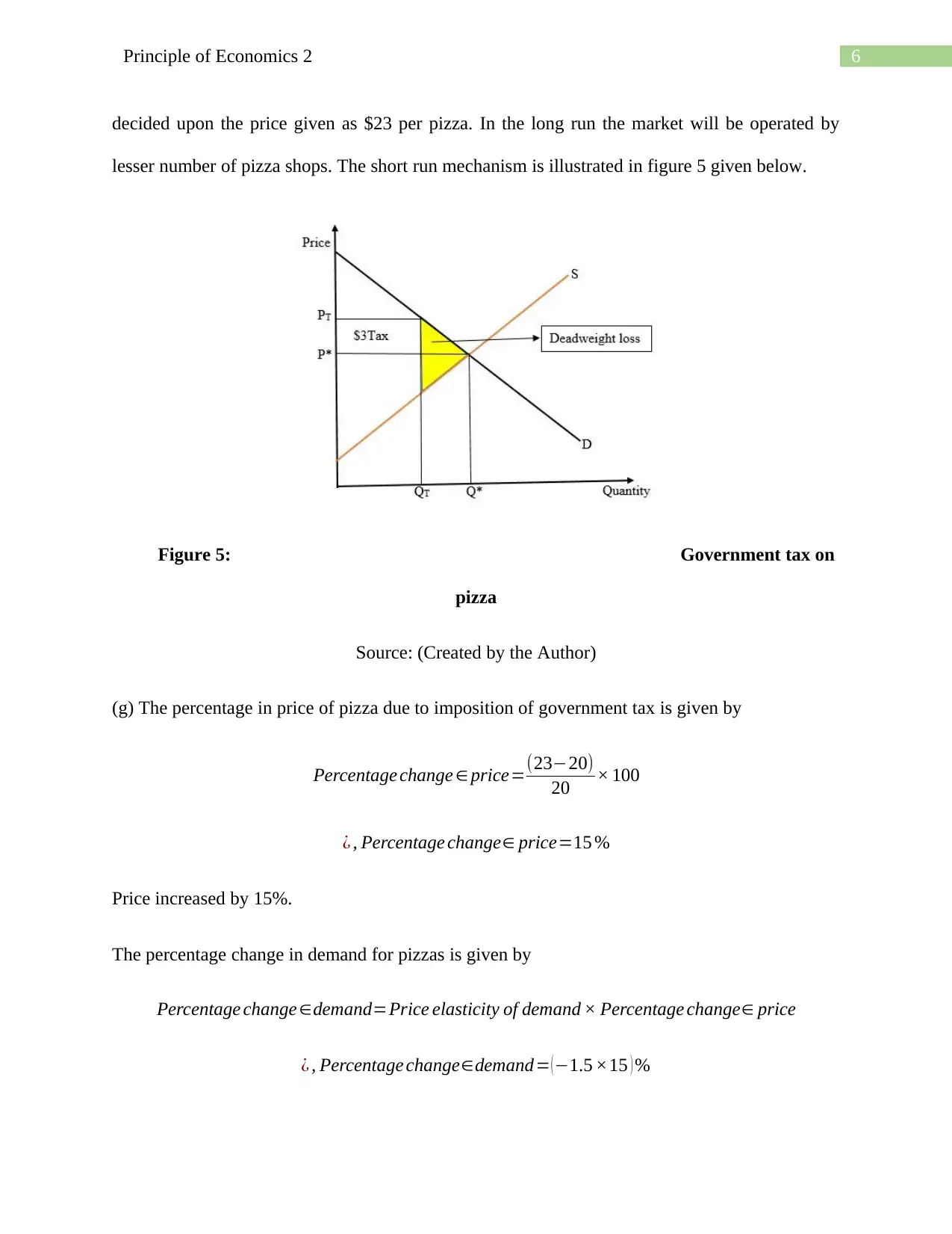
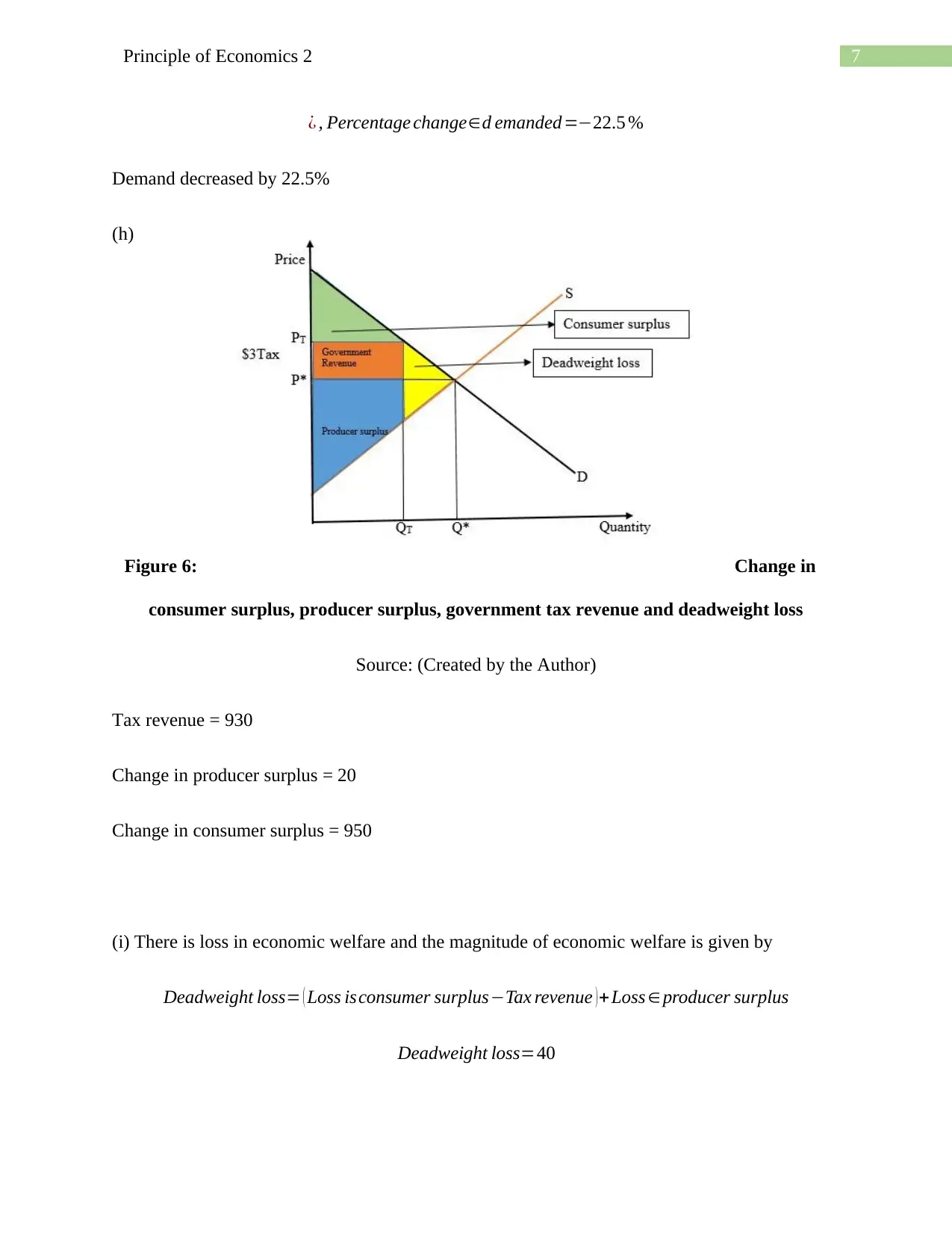
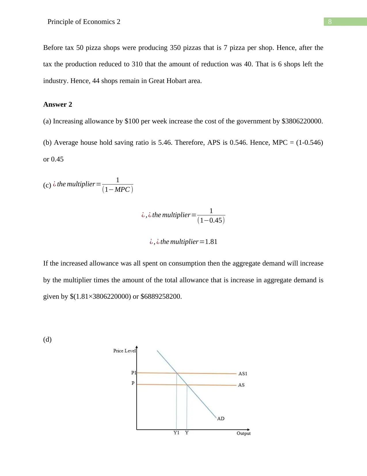
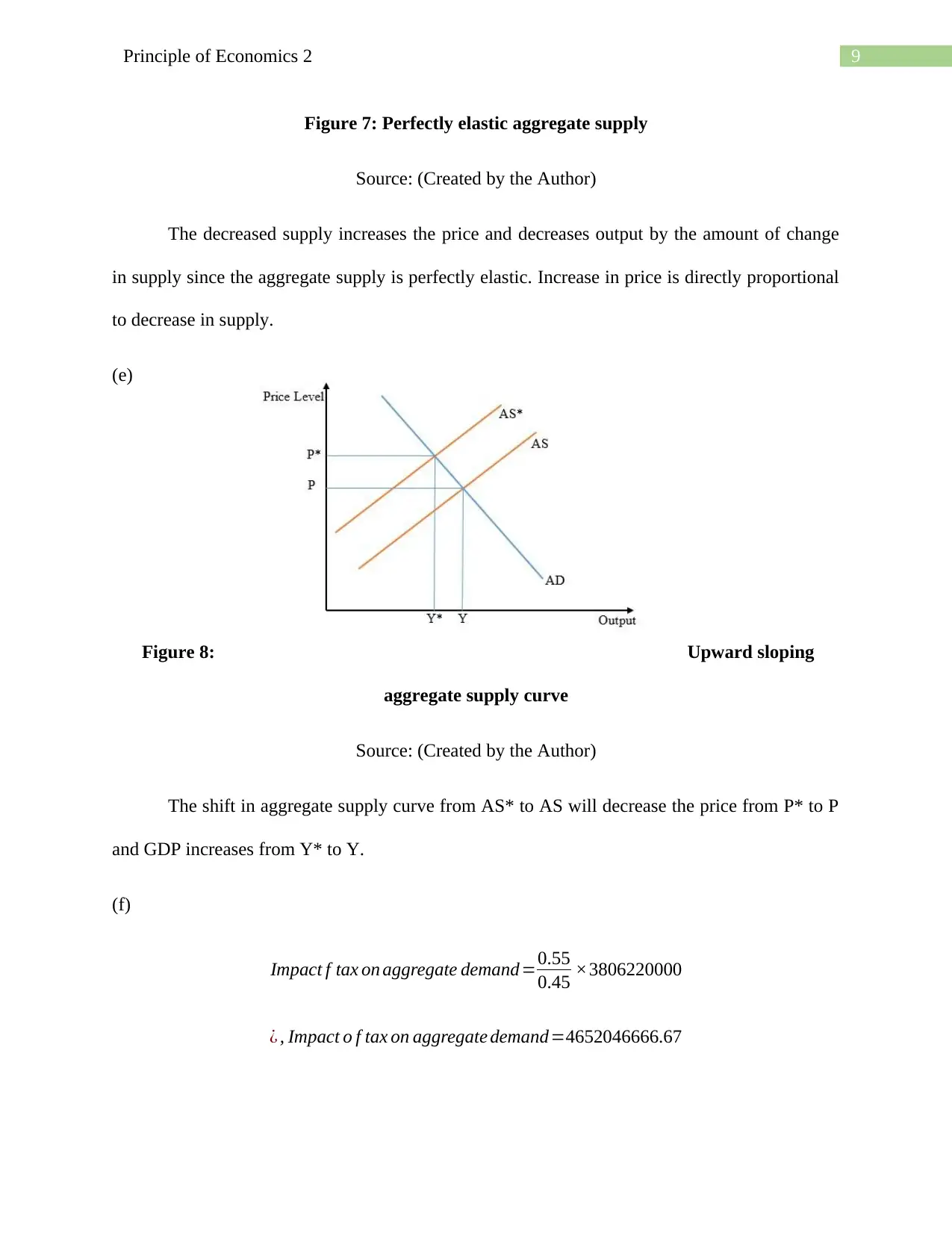
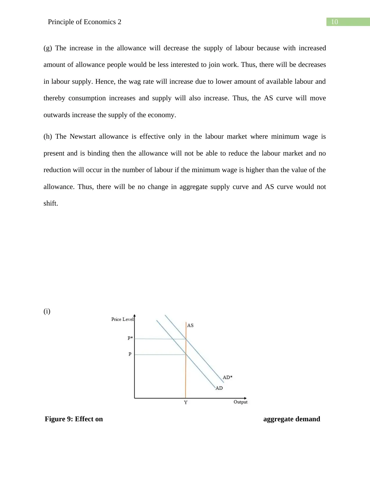
This assignment solution for BEA121 Principles of Economics 2 at the University of Tasmania addresses two main economic scenarios. The first part analyzes a pizza market, exploring cost curves, profit maximization, long-run equilibrium, the impact of price changes, and the effects of a government ta...Read More

Running head: Principle of Economics 2
Principle of Economics 2
Name of the Student
Name of the University
Student ID

1Principle of Economics 2
Table of Contents
Answer 1..........................................................................................................................................2
Answer 2..........................................................................................................................................8
References......................................................................................................................................12

2Principle of Economics 2
Answer 1
(a)
Figure 1: Average cost, marginal cost and price
Source: (Created by the Author)
(b)
50 100 150 200 250 300 350 400 450
0
5
10
15
20
25
30
35
40
45
Average cost Marginal cost Price ($)
Pizza-350
Worker -
5

3Principle of Economics 2
Figure 2:
Profit maximizing output and worker
Source: (Created by the Author)
(c) At profit maximizing output the firm’s economic profit is $1480
(d) In the long run the, the pizza shops with identical cost structure and zero barriers to entry and
exit, the firms will operate at minimum of long run average cost and charges price where it
equals average cost, marginal cost, marginal revenue and average revenue. Thus, in long run
pizza firms will make zero economic profit. The number of pizza produced and number of
workers respectively will decreases and equilibrium occurs at the minimum point of LAC. The
graphical illustration is given below in figure 3.
50 100 150 200 250 300 350 400 450
0
5
10
15
20
25
30
35
40
45
Average cost Marginal cost Price ($)

4Principle of Economics 2
Figure 3: Long run pizza
market
Source: (Created by the Author)
The price of pizza may either fall or rise in the long run and depending on the price level
other factors will change in the market. Price P1 in figure 4 is above the long run market
equilibrium price and thus expecting of earning supernormal profit new firms will enter the
market. As a result more number of workers will be hired and thus more quantity of pizza will be
produced and the price will fall to long run perfect competition equilibrium. On the other hand, if
the price is at P2, below P* shown in figure 4, then the firms in the market will make loss as the
price is below the long run average cost. Therefore, firms will make exit from the market
reducing the amount of pizza in the market and also the number of workers will decrease. Thus,
the price will rise and reaches long run perfect competition equilibrium. This market mechanism
is shown in figure 4

5Principle of Economics 2
Figure 4: Effect of price change
Source: (Created by the Author)
(e) Demand for pizzas drop during the Taste of Tasmania and the price thus drops to $13. At this
price the firm makes losses, however, the price is higher than the minimum average cost (Luo et
al. 2015). Thus, the firm by operating can cover the cost and hence will continue to operate. On
the other hand, if the is sunny during the Taste of Tasmania the price of pizza will further reduce
to $11.50. At this price the pizza shops will male loss and also will not be able cover the average
cost because the price is lower than the minimum value of average cost. Thus, the pizza shop
will be shut down.
(f) A government takeaway tax of $3 pizza will increase the buying price to the consumers from
$20 to $23. Thus, due to rise in price the consumption will decrease and equilibrium quantity fall
from Q* to QT. Thus, the revenue of the shops will decrease and many shops that are not able to
cover its cost might make exit from the market. On the other hand, in the long run the demand
will fall causing the demand curve to shift leftward and the equilibrium of the pizza market will

6Principle of Economics 2
decided upon the price given as $23 per pizza. In the long run the market will be operated by
lesser number of pizza shops. The short run mechanism is illustrated in figure 5 given below.
Figure 5: Government tax on
pizza
Source: (Created by the Author)
(g) The percentage in price of pizza due to imposition of government tax is given by
Percentage change ∈ price=(23−20)
20 × 100
¿ , Percentage change∈ price=15 %
Price increased by 15%.
The percentage change in demand for pizzas is given by
Percentage change ∈demand=Price elasticity of demand × Percentage change∈ price
¿ , Percentage change∈demand= ( −1.5 ×15 ) %

7Principle of Economics 2
¿ , Percentage change∈d emanded=−22.5 %
Demand decreased by 22.5%
(h)
Figure 6: Change in
consumer surplus, producer surplus, government tax revenue and deadweight loss
Source: (Created by the Author)
Tax revenue = 930
Change in producer surplus = 20
Change in consumer surplus = 950
(i) There is loss in economic welfare and the magnitude of economic welfare is given by
Deadweight loss= ( Loss isconsumer surplus−Tax revenue )+ Loss ∈ producer surplus
Deadweight loss=40

8Principle of Economics 2
Before tax 50 pizza shops were producing 350 pizzas that is 7 pizza per shop. Hence, after the
tax the production reduced to 310 that the amount of reduction was 40. That is 6 shops left the
industry. Hence, 44 shops remain in Great Hobart area.
Answer 2
(a) Increasing allowance by $100 per week increase the cost of the government by $3806220000.
(b) Average house hold saving ratio is 5.46. Therefore, APS is 0.546. Hence, MPC = (1-0.546)
or 0.45
(c) ¿ the multiplier= 1
(1−MPC )
¿ , ¿ the multiplier= 1
(1−0.45)
¿ , ¿ the multiplier=1.81
If the increased allowance was all spent on consumption then the aggregate demand will increase
by the multiplier times the amount of the total allowance that is increase in aggregate demand is
given by $(1.81×3806220000) or $6889258200.
(d)

9Principle of Economics 2
Figure 7: Perfectly elastic aggregate supply
Source: (Created by the Author)
The decreased supply increases the price and decreases output by the amount of change
in supply since the aggregate supply is perfectly elastic. Increase in price is directly proportional
to decrease in supply.
(e)
Figure 8: Upward sloping
aggregate supply curve
Source: (Created by the Author)
The shift in aggregate supply curve from AS* to AS will decrease the price from P* to P
and GDP increases from Y* to Y.
(f)
Impact f tax on aggregate demand=0.55
0.45 ×3806220000
¿ , Impact o f tax on aggregate demand=4652046666.67

10Principle of Economics 2
(g) The increase in the allowance will decrease the supply of labour because with increased
amount of allowance people would be less interested to join work. Thus, there will be decreases
in labour supply. Hence, the wag rate will increase due to lower amount of available labour and
thereby consumption increases and supply will also increase. Thus, the AS curve will move
outwards increase the supply of the economy.
(h) The Newstart allowance is effective only in the labour market where minimum wage is
present and is binding then the allowance will not be able to reduce the labour market and no
reduction will occur in the number of labour if the minimum wage is higher than the value of the
allowance. Thus, there will be no change in aggregate supply curve and AS curve would not
shift.
(i)
Figure 9: Effect on aggregate demand

11Principle of Economics 2
Source: (Created by the Author)
The policy will be effective only when the inflation rate is low because in long run
aggregate supply is perfectly inelastic and the effect of the policy would change the aggregate
demand only and it will directly affect price level and that would to raise the price form P to P*
(Rao 2016). As a result the inflation rate will increase.
(j) Newstart, Rental Assistance and other supplements will be shifted out of poverty if Newstart
allowance was increased by $100 a week.
0.208 million people will be lifted out of poverty. After lifting 0.208 million people out
of poverty the number of people in Australia below poverty line are (3.05-0.208) million or
2.842 million. Therefore, new poverty rate of Australia is
Poverty rate=2.842
23.1 × 100
Poverty rate=12.30 %

12Principle of Economics 2
References
Luo, X., Stordal, A.S., Lorentzen, R.J. and Nævdal, G., 2015. Iterative ensemble smoothing as an
approximation solution to a regularized minimum-average-cost problem: theory and
applications. arXiv preprint arXiv:1505.01135.
Rao, B.B. ed., 2016. Aggregate demand and supply: a critique of orthodox macroeconomic
modelling. Springer.