Principles of Economics: Macroeconomics Assignment, Term 1, 2019

This document presents a comprehensive solution to a macroeconomics assignment, addressing various key concepts and problems. The solution begins with a comparison of nominal and real GDP, demonstrating their calculation and implications. It then delves into labor economics, analyzing marginal product, labor demand under different price scenarios, and the impact of productivity changes. Further, the assignment explores the decision-making process of buying versus renting a house, considering factors like interest rates, house prices, and rent costs. Finally, the solution tackles macroeconomic equilibrium, including the calculation of autonomous expenditure, the output gap, and the effects of shifts in aggregate demand due to changes in consumer spending and negative inflation shocks, with graphical representations and policy recommendations.

MACROECONOMICS
STUDENT ID:
[Pick the date]

Question 1
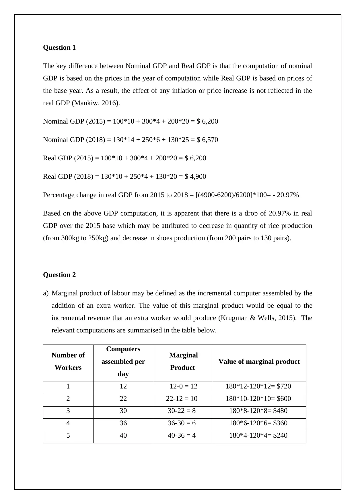
The key difference between Nominal GDP and Real GDP is that the computation of nominal
GDP is based on the prices in the year of computation while Real GDP is based on prices of
the base year. As a result, the effect of any inflation or price increase is not reflected in the
real GDP (Mankiw, 2016).
Nominal GDP (2015) = 100*10 + 300*4 + 200*20 = $ 6,200
Nominal GDP (2018) = 130*14 + 250*6 + 130*25 = $ 6,570
Real GDP (2015) = 100*10 + 300*4 + 200*20 = $ 6,200
Real GDP (2018) = 130*10 + 250*4 + 130*20 = $ 4,900
Percentage change in real GDP from 2015 to 2018 = [(4900-6200)/6200]*100= - 20.97%
Based on the above GDP computation, it is apparent that there is a drop of 20.97% in real
GDP over the 2015 base which may be attributed to decrease in quantity of rice production
(from 300kg to 250kg) and decrease in shoes production (from 200 pairs to 130 pairs).
Question 2
a) Marginal product of labour may be defined as the incremental computer assembled by the
addition of an extra worker. The value of this marginal product would be equal to the
incremental revenue that an extra worker would produce (Krugman & Wells, 2015). The
relevant computations are summarised in the table below.
Number of
Workers
Computers
assembled per
day
Marginal
Product Value of marginal product
1 12 12-0 = 12 180*12-120*12= $720
2 22 22-12 = 10 180*10-120*10= $600
3 30 30-22 = 8 180*8-120*8= $480
4 36 36-30 = 6 180*6-120*6= $360
5 40 40-36 = 4 180*4-120*4= $240

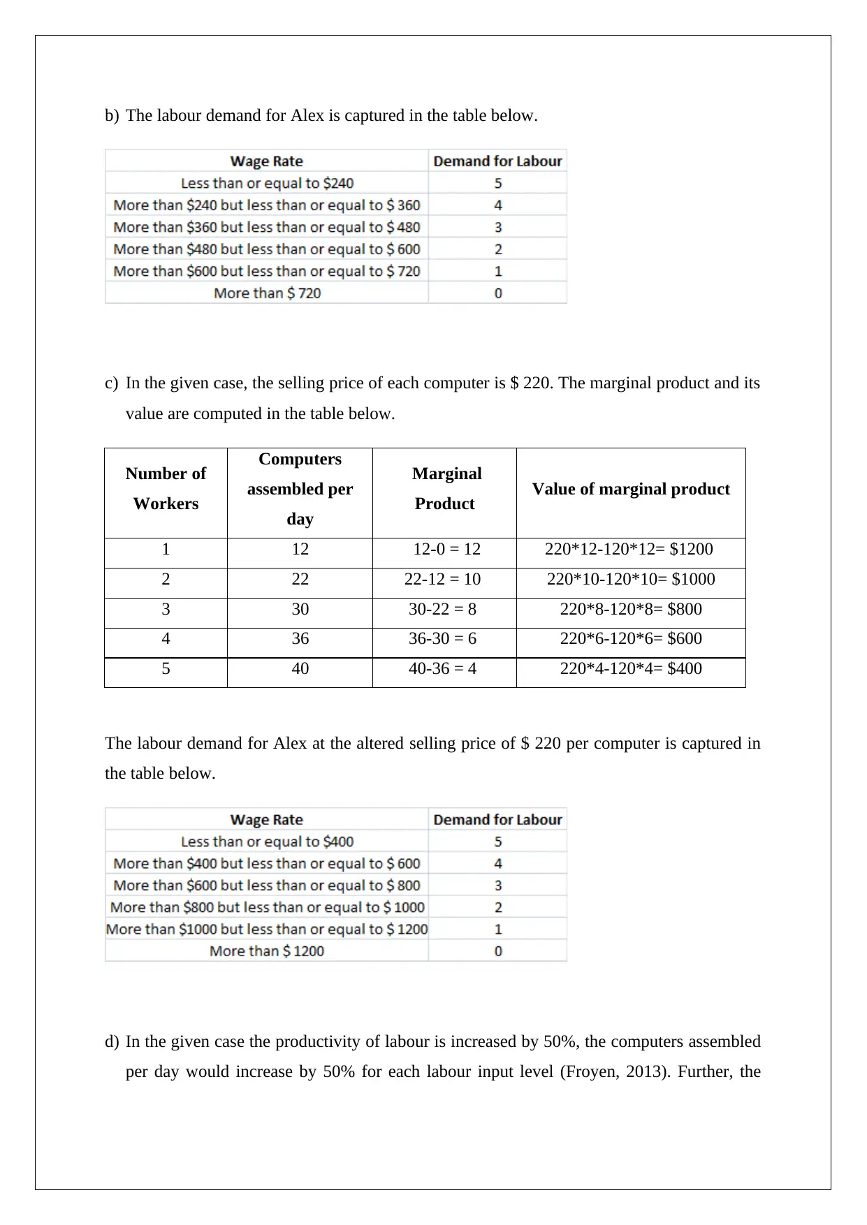
b) The labour demand for Alex is captured in the table below.
c) In the given case, the selling price of each computer is $ 220. The marginal product and its
value are computed in the table below.
Number of
Workers
Computers
assembled per
day
Marginal
Product Value of marginal product
1 12 12-0 = 12 220*12-120*12= $1200
2 22 22-12 = 10 220*10-120*10= $1000
3 30 30-22 = 8 220*8-120*8= $800
4 36 36-30 = 6 220*6-120*6= $600
5 40 40-36 = 4 220*4-120*4= $400
The labour demand for Alex at the altered selling price of $ 220 per computer is captured in
the table below.
d) In the given case the productivity of labour is increased by 50%, the computers assembled
per day would increase by 50% for each labour input level (Froyen, 2013). Further, the

selling price of the computer is $ 200 per unit. The marginal product and its value are
computed in the table below.
Number of
Workers
Computers
assembled per
day
Marginal
Product Value of marginal product
1 18 18-0 = 18 200*18-120*18= $1440
2 33 33-18 = 15 200*15-120*15= $1300
3 45 45-33 = 12 200*12-120*12= $960
4 54 54-45 = 9 200*9-120*9= $720
5 60 60-54 = 6 200*6-120*6= $480
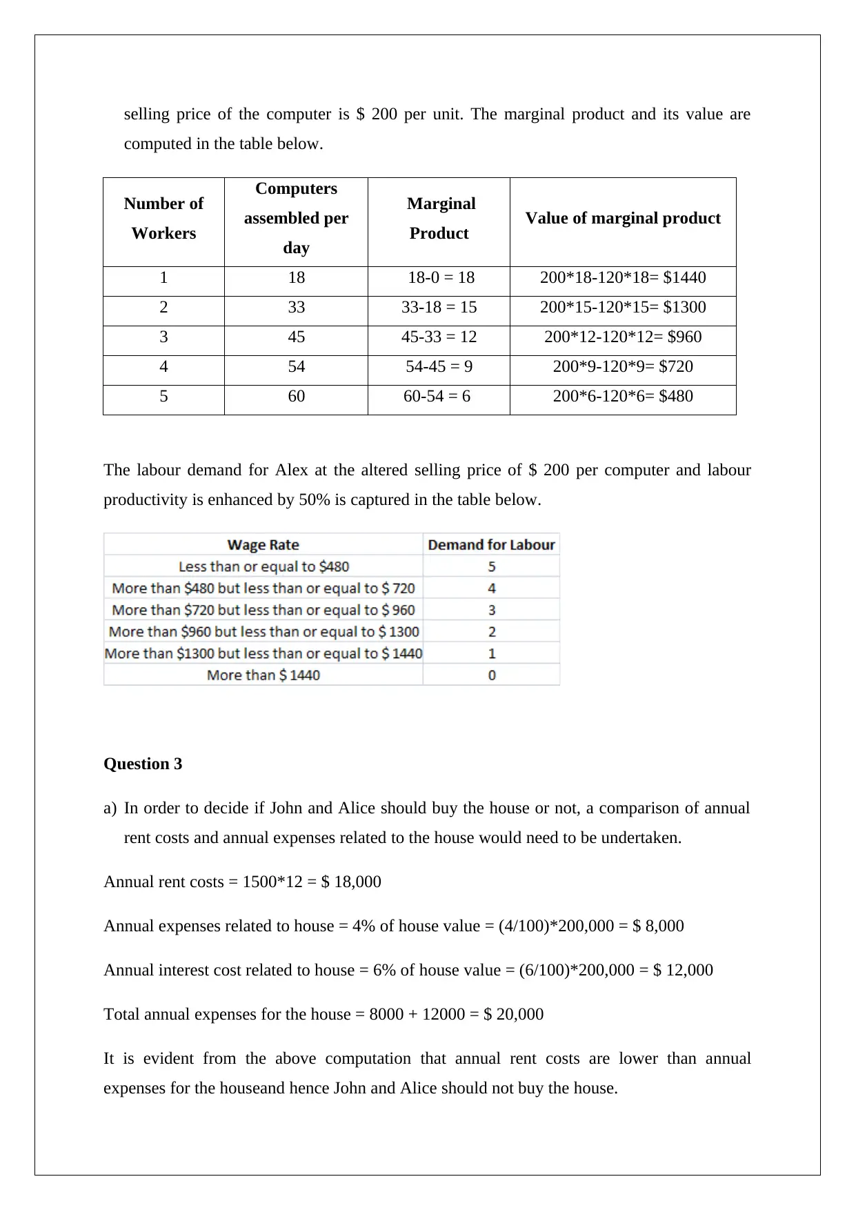
The labour demand for Alex at the altered selling price of $ 200 per computer and labour
productivity is enhanced by 50% is captured in the table below.
Question 3
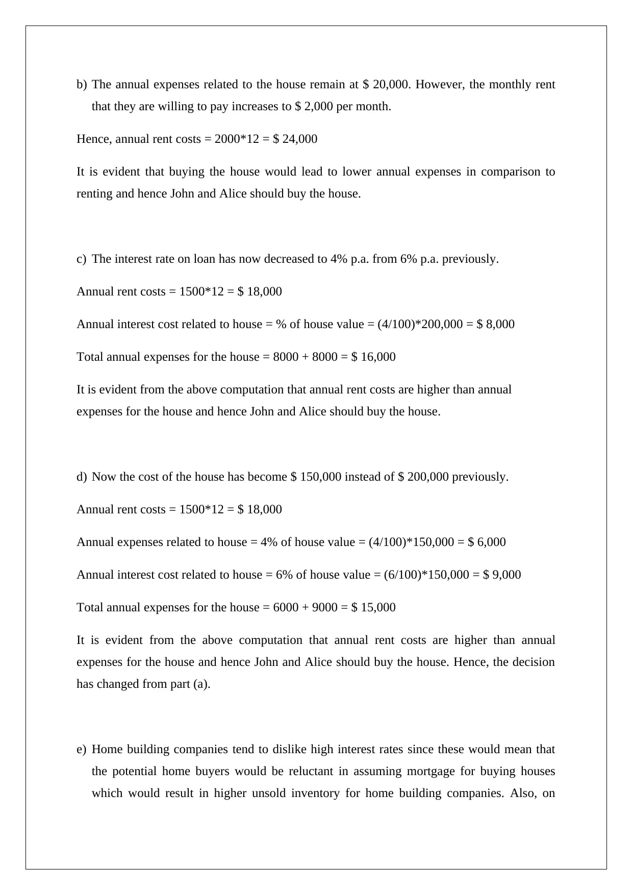
a) In order to decide if John and Alice should buy the house or not, a comparison of annual
rent costs and annual expenses related to the house would need to be undertaken.
Annual rent costs = 1500*12 = $ 18,000
Annual expenses related to house = 4% of house value = (4/100)*200,000 = $ 8,000
Annual interest cost related to house = 6% of house value = (6/100)*200,000 = $ 12,000
Total annual expenses for the house = 8000 + 12000 = $ 20,000
It is evident from the above computation that annual rent costs are lower than annual
expenses for the houseand hence John and Alice should not buy the house.

b) The annual expenses related to the house remain at $ 20,000. However, the monthly rent
that they are willing to pay increases to $ 2,000 per month.
Hence, annual rent costs = 2000*12 = $ 24,000
It is evident that buying the house would lead to lower annual expenses in comparison to
renting and hence John and Alice should buy the house.
c) The interest rate on loan has now decreased to 4% p.a. from 6% p.a. previously.
Annual rent costs = 1500*12 = $ 18,000
Annual interest cost related to house = % of house value = (4/100)*200,000 = $ 8,000
Total annual expenses for the house = 8000 + 8000 = $ 16,000
It is evident from the above computation that annual rent costs are higher than annual
expenses for the house and hence John and Alice should buy the house.
d) Now the cost of the house has become $ 150,000 instead of $ 200,000 previously.
Annual rent costs = 1500*12 = $ 18,000
Annual expenses related to house = 4% of house value = (4/100)*150,000 = $ 6,000
Annual interest cost related to house = 6% of house value = (6/100)*150,000 = $ 9,000
Total annual expenses for the house = 6000 + 9000 = $ 15,000
It is evident from the above computation that annual rent costs are higher than annual
expenses for the house and hence John and Alice should buy the house. Hence, the decision
has changed from part (a).
e) Home building companies tend to dislike high interest rates since these would mean that
the potential home buyers would be reluctant in assuming mortgage for buying houses
which would result in higher unsold inventory for home building companies. Also, on

account of lower demand of new homes from customers, there would be fall in the prices
besides a fall in the business as the new homes construction would slow down so that the
available inventory is absorbed.
Question 4
a) PAE= C+ IP + G + NX = 6000 + 0.5(Y-4000) + 2,000 + 4,500 + 500 = 11,000 + 0.5Y
From the above equation, autonomous expenditure = $ 11,000
Multiplier = 1/(1-MPC) = 1/(1-0.5) = 2
For equilibrium, Y = C + IP + G + NX
Hence, Y = 11000 + 0.5Y
Solving the above, Y = $ 22,000
The potential GDP is given as $ 21,000 and hence the output gap is ($22,000-$ 21,000) =
$1,000
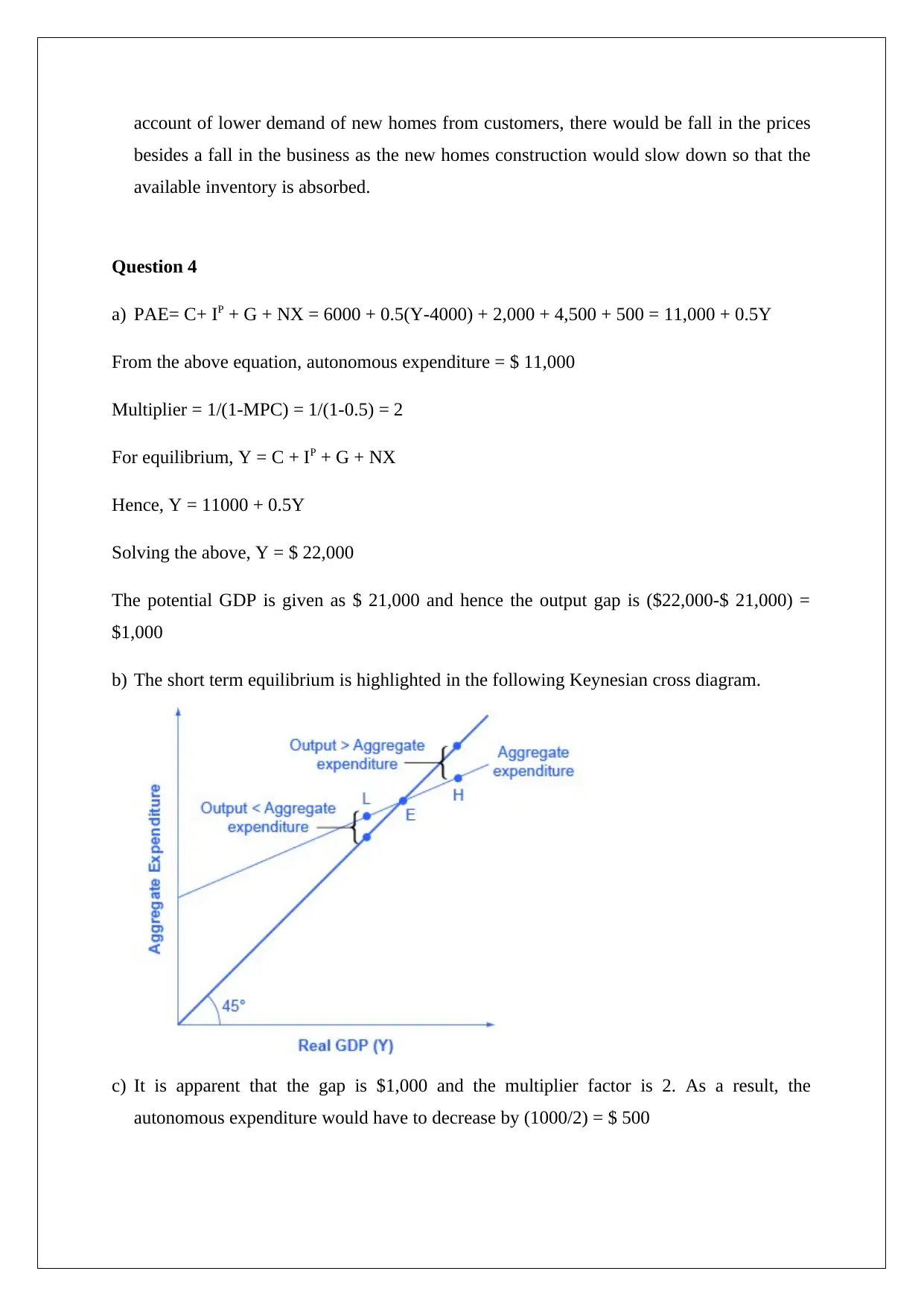
b) The short term equilibrium is highlighted in the following Keynesian cross diagram.
c) It is apparent that the gap is $1,000 and the multiplier factor is 2. As a result, the
autonomous expenditure would have to decrease by (1000/2) = $ 500

d) If the government decides to fill the output gap by increasing taxes, then the same needs to
be increased by $ 1,000 so that the output gap becomes zero. Thus, the amount of tax
would change from $ 4,000 to $ 5,000.
Question 5
a) The decline in consumer spending would tend to shift the AD curve to the left. This is
because consumer spending is one of the key components of aggregate demand. Further,
the lower consumer spending would tend to lower the demand of various goods and
services by the consumers which would be reflected in leftwards shift of AD
(McConnell, ,Brue & Flynn, 2014).
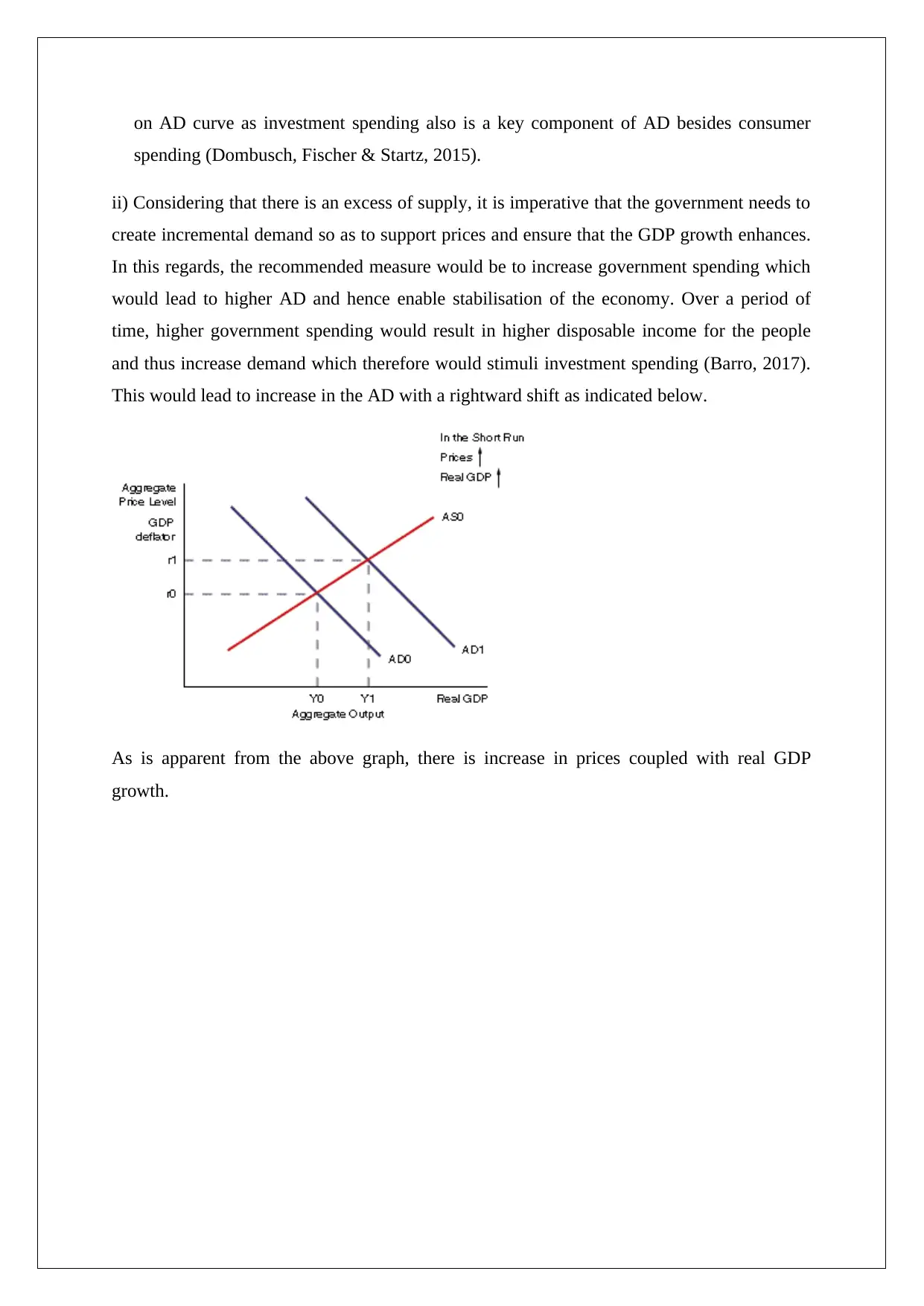
b) The impact on the short term equilibrium on account of the above described AD curve
shift is summarised below.
There is a shift of AD curve from AD1 to AD2. In the short run, there is no change in the
aggregate supply which remains as the previous level as AS. The result is that there is a
decrease in both equilibrium price and also equilibrium real GDP. Hence, in the short run
owing to lesser AD, the prices would become lower and also real GDP growth would be
adversely impacted (Koutsoyiannis,2013).
c) (i) On account of the negative inflation shock, there would be a fall in the prices which
reflects that the supply is significantly higher than the corresponding demand. As a result,
the investment spending would be adversely impacted as there would be lower capacity
utilisation and hence the installation of new capacities would be deferred. Thus, there
would be lowering of investment spending which would have additional adverse impact

on AD curve as investment spending also is a key component of AD besides consumer
spending (Dombusch, Fischer & Startz, 2015).
ii) Considering that there is an excess of supply, it is imperative that the government needs to
create incremental demand so as to support prices and ensure that the GDP growth enhances.
In this regards, the recommended measure would be to increase government spending which
would lead to higher AD and hence enable stabilisation of the economy. Over a period of
time, higher government spending would result in higher disposable income for the people
and thus increase demand which therefore would stimuli investment spending (Barro, 2017).
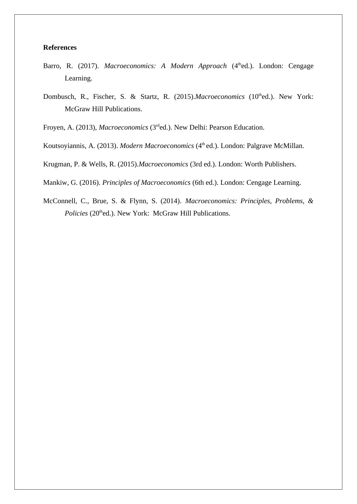
This would lead to increase in the AD with a rightward shift as indicated below.
As is apparent from the above graph, there is increase in prices coupled with real GDP
growth.

References
Barro, R. (2017). Macroeconomics: A Modern Approach (4thed.). London: Cengage
Learning.
Dombusch, R., Fischer, S. & Startz, R. (2015).Macroeconomics (10thed.). New York:
McGraw Hill Publications.
Froyen, A. (2013), Macroeconomics (3rded.). New Delhi: Pearson Education.
Koutsoyiannis, A. (2013). Modern Macroeconomics (4th ed.). London: Palgrave McMillan.
Krugman, P. & Wells, R. (2015).Macroeconomics (3rd ed.). London: Worth Publishers.
Mankiw, G. (2016). Principles of Macroeconomics (6th ed.). London: Cengage Learning.
McConnell, C., Brue, S. & Flynn, S. (2014). Macroeconomics: Principles, Problems, &
Policies (20thed.). New York: McGraw Hill Publications.