Probability and Statistics: Assignment 1, Analysis and Calculations

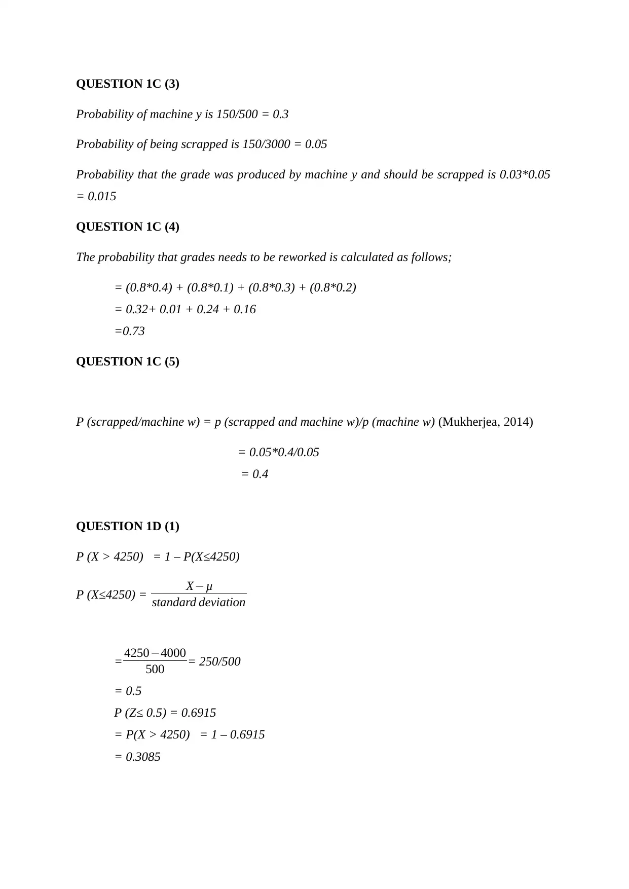
This document presents a complete solution for a probability and statistics homework assignment. The assignment covers several key concepts, including the definition and calculation of expected value within a discrete probability distribution, demonstrated through a practical example. It includes a detailed analysis of daily sales data, requiring the completion of a table with formulas to calculate cumulative probabilities, variance, and standard deviation. The solution also addresses probability calculations related to machine production and rework, as well as problems involving normal distribution. Finally, the assignment concludes with data analysis of population statistics and confidence interval calculations.

QUESTION 1A
Expected value is simply referred as the mean and it measures the average of numbers of
numbers or units (Virah sahn, 2011)
According to (Bin Zhao, 2012), It is computed as ∑ x p (x)where x is a discrete random
variable and p(x) is the probability of the discrete random variable x
Example
x P(x)
0 0.1
1 0.2
2 0.4
3 0.3
P(x) = ∑ x p (x)
= x p ( X =0 ) + x p ( X =1 ) + x p ( X =2 ) + x p( X=3)
=0*0.1 + 1*0.2 + 2*0.4 + 3*0.3
=1.9
QUESTION 1B (1)
SALES
UNIT (X)
NUMBER
OF DAYS P(X)
EXP
VALUE
MORE
THAN
LESS
THAN [X-E(X)] ^2 [X-[E(X)] ^2P(X)]
0 5 0.05 0 0.95 0.05 8.41 0.4205
1 10 0.1 0.1 0.85 0.15 3.61 0.361
2 25 0.25 0.5 0.6 0.4 0.81 0.2025
3 25 0.25 0.75 0.35 0.65 0.01 0.0025
4 20 0.2 0.8 0.15 0.85 1.21 0.242
5 15 0.15 0.75 0 1 4.41 0.6615
TOTAL 100 1 2.9
p(x≥2) =
0.6
p(x≤3)
=0.65 VARIANCE 1.89
STANDARD
DEVIATION 1.374772708

QUESTION 1B (2)
The average daily sales
E(X) = X1P1 + X2P2 + X3P3 + X4P4 + X5P5 + X6P6
= 0*0 + 1*0.1 + 2* 0.5 + 3* 0.75 + 4* 0.8 + 5* 0.75
= 2.9
QUESTION 1B (3)
P (x ≥ 2) = 1 – p (x ≤ 2)
= 1 – (p(x=0) + p (x =1) + p (x =2))
=1 – (0.05 + 0.1 + 0.25)
=1- 0.4
=0.6
QUESTION 1B (4)
p (x ≤ 3)
=p(x=0) + p(x=1) + p(x=2) + p(x=3)
=0.05 + 0.1 + 0.25 + 0.25
= 0.65
QUESTION 1B (5)
The variance is 1.89
Sum([X-[E(X)]2P(X)])
=8.41*0.05 + 3.61*0.1 + 0.81*0.25 + 0.01*0.25 + 1.21*0.2 + 4.41*0.15

=0.4205 + 0.361 + 0.2025 + 0.0025 + 0.242 + 0.66
= 1.89
QUESTION 1B (6)
Standard deviation is 1.374772708
= sqrt (8.41*0.05 + 3.61*0.1 + 0.81*0.25 + 0.01*0.25 + 1.21*0.2 + 4.41*0.15)
=sqrt (0.4205 + 0.361 + 0.2025 + 0.0025 + 0.242 + 0.66)
=sqrt (1.89)
=1.374772708
QUESTION 1C (1)
Probability of machine W is 3200/8000 = 0.15
Probability of rework on w is 600/4000 =0.4
Therefore, the probability being produced by machine w and should be reworked is (Ryan,
2013)0.15*0.4 = 0.06
QUESTION 1C (2)
Probability that machine Z is picked is 1600/8000 = 0.8
The probability that the grade is satisfactory is 3200/4000 = 0.4
The probability of not being satisfactory is therefore 1-0.4 = 0.6
Therefore, the probability that the grade was produced by a part Z and was not satisfactory
is calculated as follows;
=0.8*0.6 = 0.48

QUESTION 1C (3)
Probability of machine y is 150/500 = 0.3
Probability of being scrapped is 150/3000 = 0.05
Probability that the grade was produced by machine y and should be scrapped is 0.03*0.05
= 0.015
QUESTION 1C (4)
The probability that grades needs to be reworked is calculated as follows;
= (0.8*0.4) + (0.8*0.1) + (0.8*0.3) + (0.8*0.2)
= 0.32+ 0.01 + 0.24 + 0.16
=0.73
QUESTION 1C (5)
P (scrapped/machine w) = p (scrapped and machine w)/p (machine w) (Mukherjea, 2014)
= 0.05*0.4/0.05
= 0.4
QUESTION 1D (1)
P (X > 4250) = 1 – P(X≤4250)
P (X≤4250) = X−μ
standard deviation
= 4250−4000
500 = 250/500
= 0.5
P (Z≤ 0.5) = 0.6915
= P(X > 4250) = 1 – 0.6915
= 0.3085

QUESTION 1D (2)
P (X < 3600) = P(X≤3600)
P (X≤3600) = 3600−4000
500
= - 0.8
P (Z≤ -0.8) = 0.2119
= 0.2119
QUESTION 1D (3)
P (X < 4500) = P(X≤4500)
P (X≤3600) = 4500−4000
500
= 1
P (Z≤ 1) = 0.8413
= 0.8413
QUESTION 2
1. The average age of the Australian population is 37.5 years
Year Population Median Age
2019 25,088,636 37.5
2018 24,772,247 37.5
2017 24,450,561 37.5
2016 24,125,848 37.5

2. The average age of male to die in Australia is 84.9 while the average age of female to
die in Australia is 87.8
Male = (80.4 + 80.7 + 80.9 + 81.2 + 82.1 + 84.6 + 91.2 + 98.0)/8 = 84.9
Female =84.6 + 84.8 + 85.0 + 85.1 + 85.6 + 87.3 + 92.3 +98.3/8 =87.8
Age (years) Males
2014–2016
Females
2014–2016
0 (birth) 80.4 84.6
1 80.7 84.8
15 80.9 85.0
25 81.2 85.1
45 82.1 85.6
65 84.6 87.3
85 91.2 92.3
95 98.0 98.3

3. The percentage of people working in Australia is 57.7%
Australia - Persons (Usual residence) 2016
Employment status Number %
Greater
Capital
Cities % Number
Employed 10,683,838 93.1 93.1 10,057,142
Employed full-time 6,623,071 57.7 58.6 6,366,682
Employed part-time 3,860,683 33.7 32.8 3,472,012
Hours worked not stated 200,084 1.7 1.7 218,448
Unemployed (Unemployment rate) 787,456 6.9 6.9 600,098
Looking for full-time work 447,652 3.9 3.8 357,833
Looking for part-time work 339,804 3.0 3.1 242,265
Total labour force 11,471,294 100.0 100.0 10,657,240
QUESTION 3(A1)
The sample = 64 observations
Mean time = 20 hrs.
Standard deviation = 5 hrs.
Therefore, to calculate the upper and lower confidence interval (TÉLLEZ ARNOLDO,
2015), we proceed as follows,
To allow for degrees of freedom, we subtract 1 from the sample observation
= 64-1

At 95% level of confidence, (1-0.95)/2 = 0.025
Checking 0.025 in the t table for 9 degree of freedom, we get 2.262
Therefore
= standard deviation/ (sqrt (sample observation))
= σ
√ sample observation
= 5
√64 = 0.625
For the lower confidence interval
Mean time – 0.625
= 20 -0.625
= 19.375
For the Upper confidence interval
Mean time – 0.625
= 20 + 0.625
= 20.625
QUESTION 3(A2)
For a sample of 9 observations,
At 95% level of confidence, (1-0.95)/2 = 0.025
σ
√ sample observation

= 5
√9
= 1.666667
For the lower confidence interval
Mean time – 1.666667
= 20 -1.666667
= 18.33333
For the Upper confidence interval
Mean time – 1.666667
= 20 + 1.666667
= 21.66667
QUESTION 3b (1)
According to (Christos Lionis, 2010), We formulate a hypothesis as follows
H0: μ ≤ m (There no age discrimination)
H1: μ ≥ m (There is age discrimination)
QUESTION 3b (2)
To calculate the critical value, (Fantz, 2010) emphasized on the steps to follow procedurally
in order to obtain the critical value. Therefore, we proceed as follows
We first compute the formula;
Z =
μ−m
σ
√ n
Z =
45−42
10.8
√ 49
=
3
10.8
7

= 3
1.542857143
= 1.9444
checking the p- value from the normal table at 5% level of significance, we obtain the p-
value to be 0.9738
The p-value is 0.9738
QUESTION 3b (3)
QUESTION 3b (4)
Since the p-value 0.9738 is greater than alpha 0.05 (Fraser, 2017) ,we fail to reject the null
hypothesis and therefore conclude that we do not have enough evidence to support the claim
that there is age discrimination.
I t therefore means that, the claim that there I age discrimination because of laying- off older
people more than the average workers is not true based on the results due to insufficient
evidence to support the claim. Therefore, we conclude that there is no age discrimination at
all.

References
Bin Zhao, X. L. (2012). Discrete time variable structure control method. Earthquake Engineering &
structural dynamics, 52-64.
Christos Lionis, D. A. (2010). Bio-psychosocial determinants of cardiovascular disease in a rural
population on Crete, Greece: formulating a hypothesis and designing the SPILI-III study.
Journal of hypothesis testing, 3(1), 2-16.
Fantz, C. (2010). Strategies for Evaluating Critical Value Limits: Opportunities for Saving Time and
Money Without Compromising Care. Critical Values, 3(1), 36-58.
Fraser, D. (2017). p -Values: The Insight to Modern Statistical Inference. Annual Review of Statistics
and Its Application, 4(1), 83-92.
Mukherjea, S. (2014). Conditional expected durations of play given the ultimate outcome for a
correlated walk. Statistics and probability letters, 104-118.
Ryan, T. (2013). Wiley series in probability and statistics. Survival Analysis and reliability, 84-96.
TÉLLEZ ARNOLDO, G. C.-V. (2015). Effect size, confidence intervals and statistical power in
psychological research. Psychology in Russia: State of the art, 8(3), 28-39.
Virah sahn, X. (2011). New expression for the expectation value integral for a confined helium atom.
Computational & Theritical chemistry, 14-22.