Decision Support Tools Assignment - Statistical Decision Making

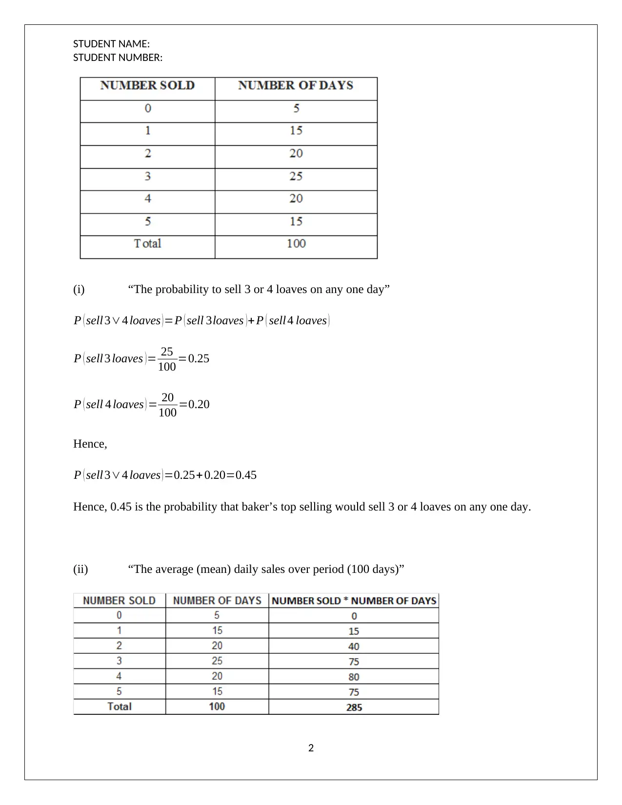
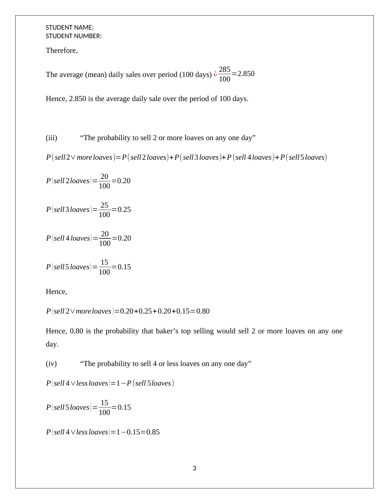
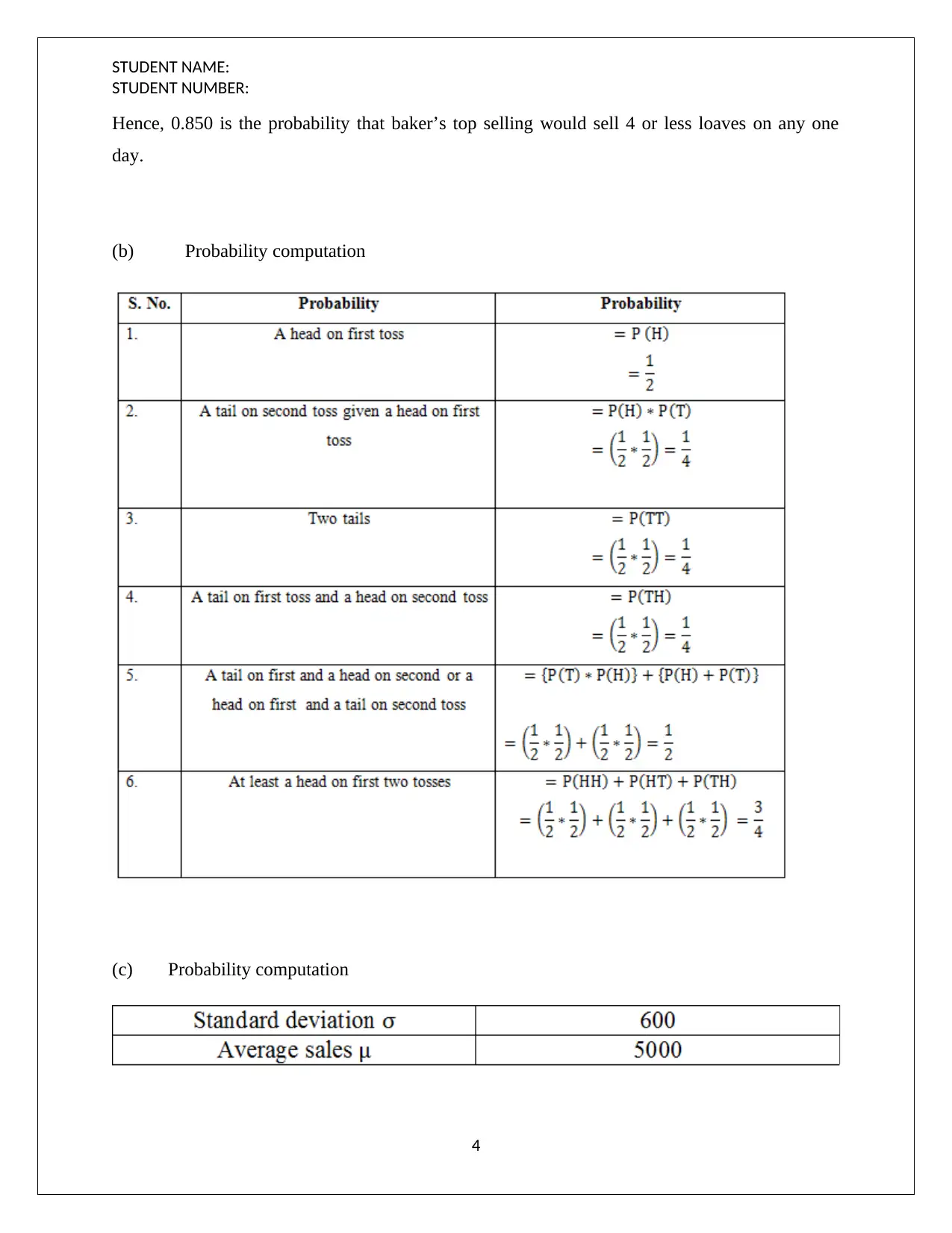
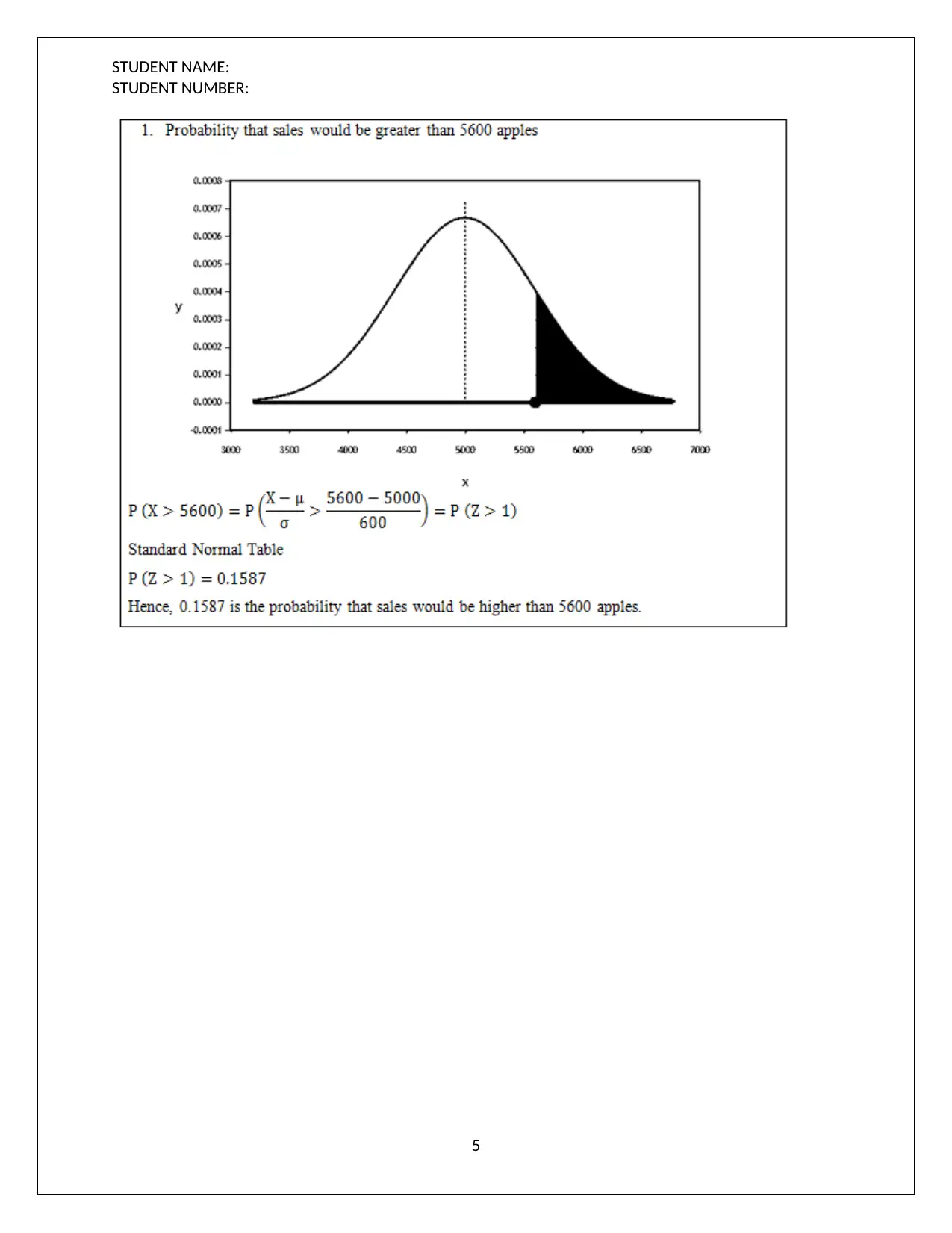
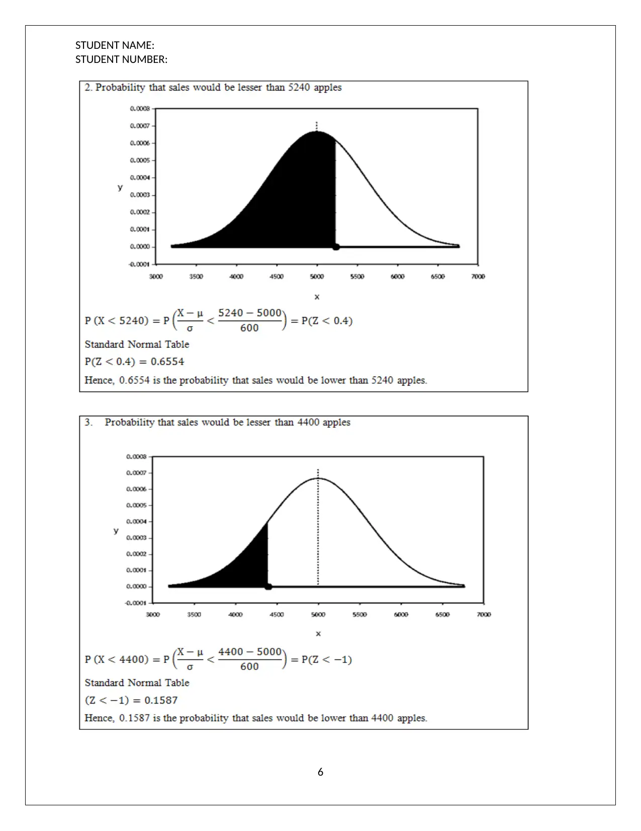
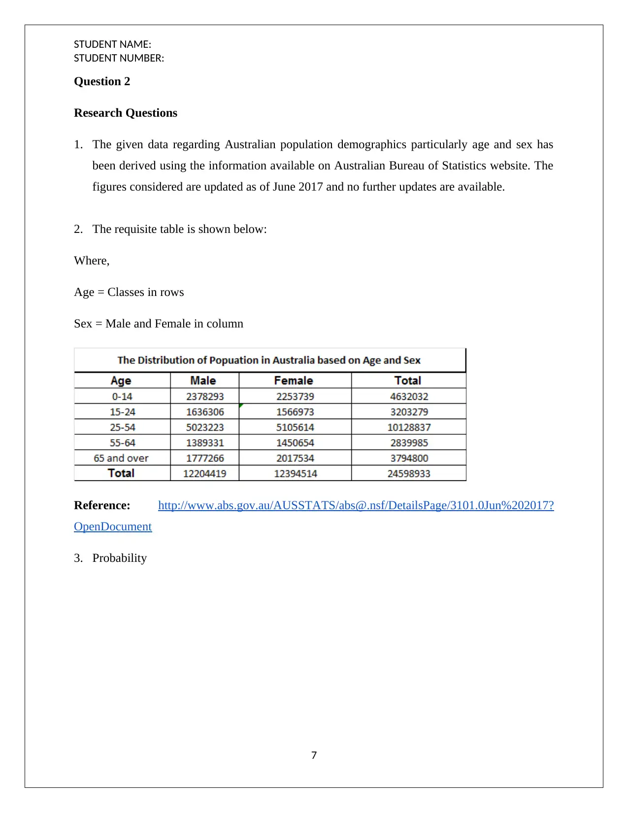
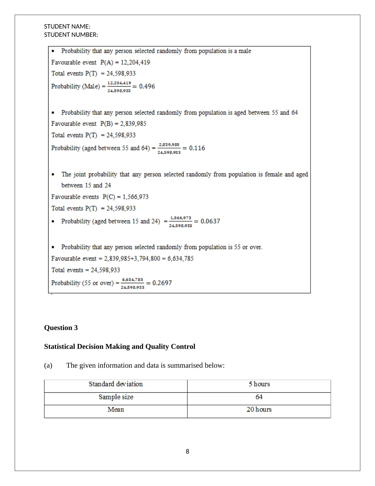
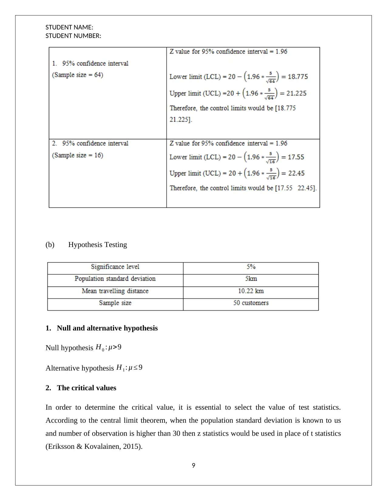
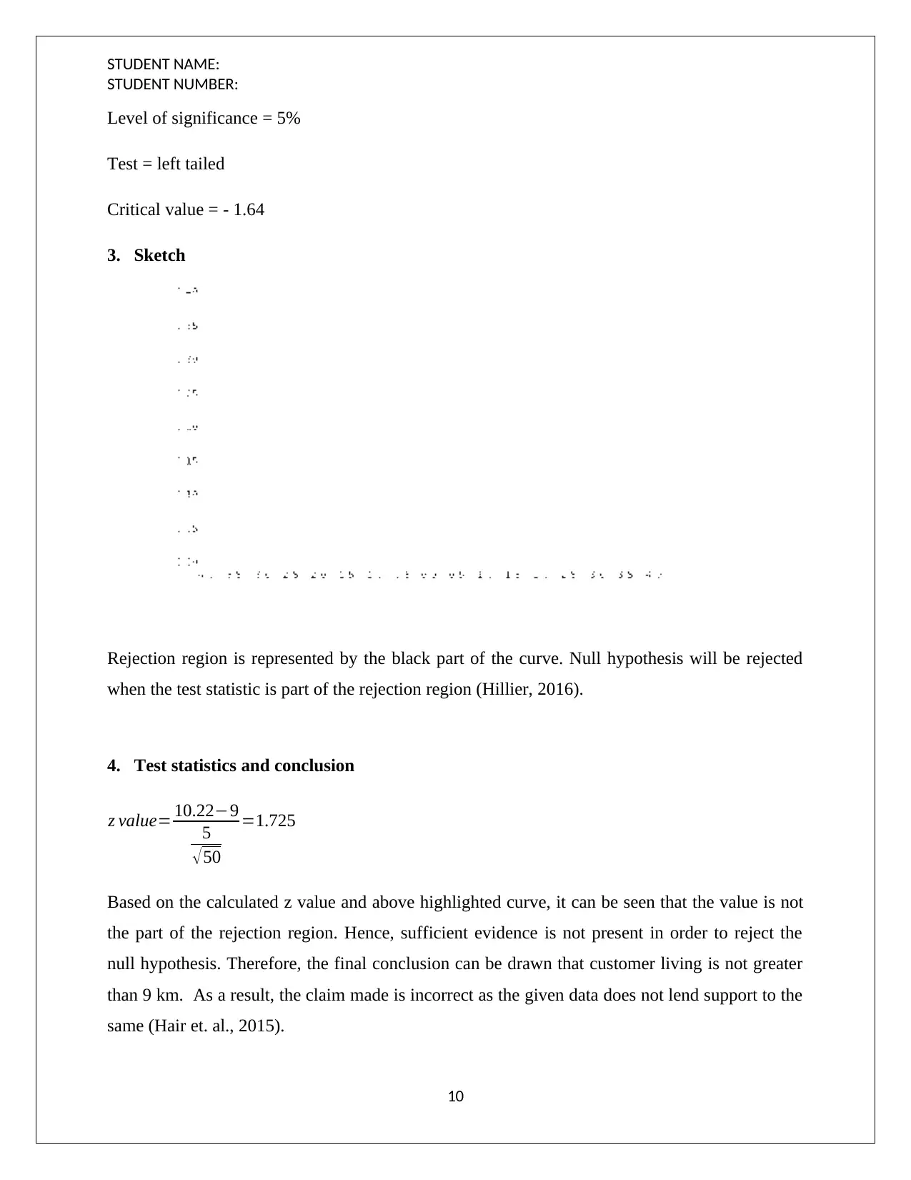
This document is a student's assignment on decision support tools, covering probability distributions, hypothesis testing, and statistical decision-making. The assignment begins with an explanation of discrete and continuous probability distributions, providing examples and calculations related to daily sales data. It then delves into research questions based on Australian population demographics, analyzing age and sex data from the Australian Bureau of Statistics. The final section focuses on statistical decision-making and quality control, including hypothesis testing, null and alternative hypotheses, critical values, and test statistics. A z-test is performed to analyze a claim, with the conclusion drawn based on the calculated z-value and rejection region. The assignment concludes with a list of relevant references.

Decision Support Tools
Assignment
Student Name
Student Id
Subject Name
Subject Code
Lecturer Name

STUDENT NAME:
STUDENT NUMBER:
Question 1
Probability
(a) Any probability distribution is essentially a statistical function capable of representing the
possible values that a given random variable can assume and also lists down the
corresponding probability for the same (Flick, 2015).
There are various differences between continuous and discrete probability distribution
which are highlighted as follows (Fehr & Grossman, 2013).
 The primary difference pertains to the random variable which is discrete for discrete
probability distribution and continuous for a continuous probability distribution.
 The representation of a continuous probability distribution is achieved through
probability density function while the same is achieved through probability mass
function in case of discrete probability distribution.
 The nature of frequency plot is continuous in case of continuous probability
distributions and the same is discrete when discrete probability distributions are
considered (Hastie, Tibshirani & Friedman, 2011).
Example:
Continuous Probability Distribution – Normal Distribution
Discrete Probability Distribution – Binomial Distribution
(a) Daily Sales with respect to number of days of selling the lead of bread is represented
below:
1

STUDENT NAME:
STUDENT NUMBER:
(i) “The probability to sell 3 or 4 loaves on any one day”
P ( sell 3∨4 loaves ) =P ( sell 3loaves ) + P ( sell 4 loaves )
P ( sell 3 loaves )= 25
100 =0.25
P ( sell 4 loaves ) = 20
100 =0.20
Hence,
P ( sell 3∨4 loaves )=0.25+0.20=0.45
Hence, 0.45 is the probability that baker’s top selling would sell 3 or 4 loaves on any one day.
(ii) “The average (mean) daily sales over period (100 days)”
2

STUDENT NAME:
STUDENT NUMBER:
Therefore,
The average (mean) daily sales over period (100 days) ¿ 285
100 =2.850
Hence, 2.850 is the average daily sale over the period of 100 days.
(iii) “The probability to sell 2 or more loaves on any one day”
P(sell 2∨more loaves)=P( sell 2 loaves)+ P(sell 3 loaves)+ P (sell 4 loaves)+ P(sell 5 loaves)
P ( sell 2loaves ) = 20
100 =0.20
P ( sell 3 loaves )= 25
100 =0.25
P ( sell 4 loaves ) = 20
100 =0.20
P ( sell 5 loaves ) = 15
100 =0.15
Hence,
P ( sell 2∨more loaves )=0.20+0.25+ 0.20+0.15=0.80
Hence, 0.80 is the probability that baker’s top selling would sell 2 or more loaves on any one
day.
(iv) “The probability to sell 4 or less loaves on any one day”
P ( sell 4∨less loaves ) =1−P (sell 5loaves)
P ( sell 5 loaves ) = 15
100 =0.15
P ( sell 4∨less loaves )=1−0.15=0.85
3

STUDENT NAME:
STUDENT NUMBER:
Hence, 0.850 is the probability that baker’s top selling would sell 4 or less loaves on any one
day.
(b) Probability computation
(c) Probability computation
4

STUDENT NAME:
STUDENT NUMBER:
5

STUDENT NAME:
STUDENT NUMBER:
6

STUDENT NAME:
STUDENT NUMBER:
Question 2
Research Questions
1. The given data regarding Australian population demographics particularly age and sex has
been derived using the information available on Australian Bureau of Statistics website. The
figures considered are updated as of June 2017 and no further updates are available.
2. The requisite table is shown below:
Where,
Age = Classes in rows
Sex = Male and Female in column
Reference: http://www.abs.gov.au/AUSSTATS/abs@.nsf/DetailsPage/3101.0Jun%202017?
OpenDocument
3. Probability
7

STUDENT NAME:
STUDENT NUMBER:
Question 3
Statistical Decision Making and Quality Control
(a) The given information and data is summarised below:
8

STUDENT NAME:
STUDENT NUMBER:
(b) Hypothesis Testing
1. Null and alternative hypothesis
Null hypothesis H0 : μ>9
Alternative hypothesis H1 : μ ≤ 9
2. The critical values
In order to determine the critical value, it is essential to select the value of test statistics.
According to the central limit theorem, when the population standard deviation is known to us
and number of observation is higher than 30 then z statistics would be used in place of t statistics
(Eriksson & Kovalainen, 2015).
9

STUDENT NAME:
STUDENT NUMBER:
Level of significance = 5%
Test = left tailed
Critical value = - 1.64
3. Sketch
Rejection region is represented by the black part of the curve. Null hypothesis will be rejected
when the test statistic is part of the rejection region (Hillier, 2016).
4. Test statistics and conclusion
z value= 10.22−9
5
√50
=1.725
Based on the calculated z value and above highlighted curve, it can be seen that the value is not
the part of the rejection region. Hence, sufficient evidence is not present in order to reject the
null hypothesis. Therefore, the final conclusion can be drawn that customer living is not greater
than 9 km. As a result, the claim made is incorrect as the given data does not lend support to the
same (Hair et. al., 2015).
10

STUDENT NAME:
STUDENT NUMBER:
References
Eriksson, P. & Kovalainen, A. (2015) Quantitative methods in business research (3rd ed.).
London: Sage Publications.
Fehr, F. H., & Grossman, G. (2013) An introduction to sets, probability and hypothesis testing
(3rd ed.). Ohio: Heath.
Flick, U. (2015) Introducing research methodology: A beginner's guide to doing a research
project (4th ed.). New York: Sage Publications.
Hair, J. F., Wolfinbarger, M., Money, A. H., Samouel, P., & Page, M. J. (2015).Essentials of
business research methods (2nd ed.). New York: Routledge.
Hastie, T., Tibshirani, R. & Friedman, J. (2011) The Elements of Statistical Learning (4th
ed.). New York: Springer Publications.
Hillier, F.(2016) Introduction to Operations Research. (6th ed.). New York: McGraw Hill
Publications.
11