Break-Even Analysis and Profit Calculation for Products A and B

The task requires computing the number of units for Products A and B needed to reach a specific profit target. Product A has a selling price of $10 per unit with a variable cost of $5, resulting in a contribution margin of $5. For Product B, which sells at $20 per unit with a variable cost of $12, the contribution margin is $8. The total fixed costs are set at $4,000. To achieve a profit before tax of $5,000, and another scenario to reach a post-tax profit of $21,000 (considering a 30% tax rate), calculations need to be done based on these parameters using a production ratio of 2:1 for Products A to B. The assignment explores concepts such as weighted average contribution margin and determining targeted sales volume under different financial objectives.

Running Head: DECISION MAKING
Decision Making
Name of the Student
Name of the University
Author Note

1DECISION MAKING
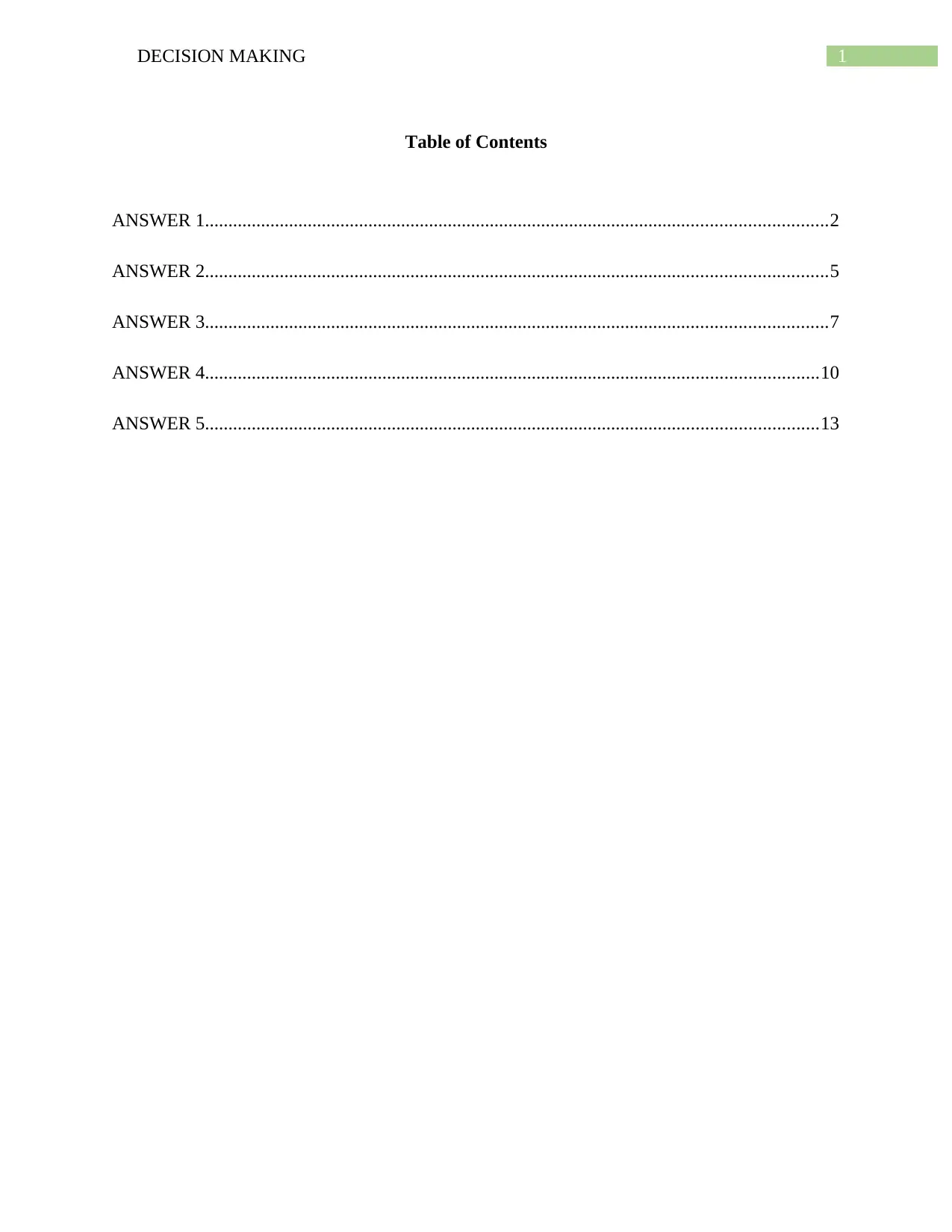
Table of Contents
ANSWER 1.....................................................................................................................................2
ANSWER 2.....................................................................................................................................5
ANSWER 3.....................................................................................................................................7
ANSWER 4...................................................................................................................................10
ANSWER 5...................................................................................................................................13

2DECISION MAKING
ANSWER 1
(a) Making a decision will be known as decision making under certainty if a person
has to make some decisions in the presence of all the necessary information.
There may be some situation when the possible decisions that can be made have a
particular probability of occurrence. Decision made under this condition is known as
decision making under risk.
Making a decision will be known as decision making under uncertainty if a
person has to make some decisions in the absence of all the necessary information.
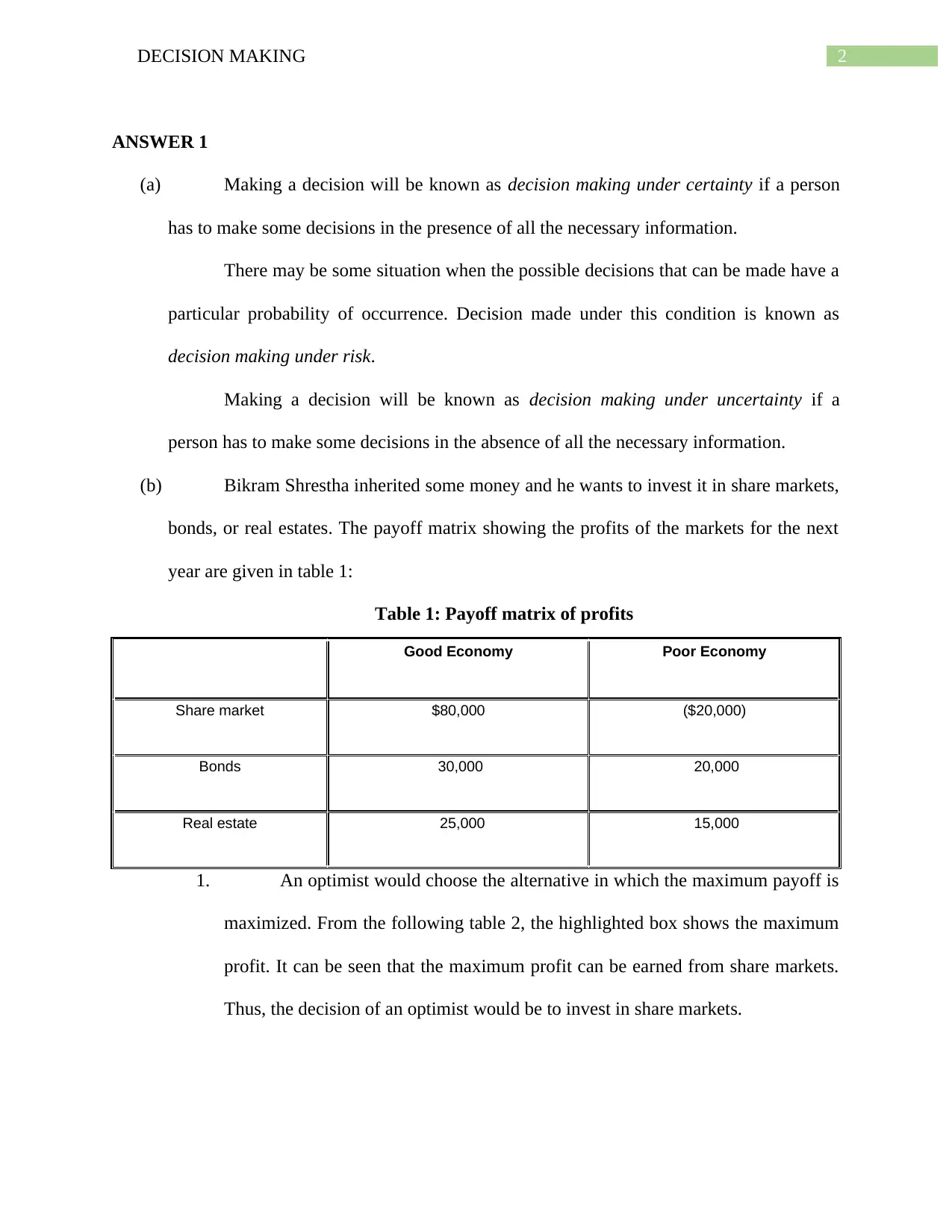
(b) Bikram Shrestha inherited some money and he wants to invest it in share markets,
bonds, or real estates. The payoff matrix showing the profits of the markets for the next
year are given in table 1:
Table 1: Payoff matrix of profits
Good Economy Poor Economy
Share market $80,000 ($20,000)
Bonds 30,000 20,000
Real estate 25,000 15,000
1. An optimist would choose the alternative in which the maximum payoff is
maximized. From the following table 2, the highlighted box shows the maximum
profit. It can be seen that the maximum profit can be earned from share markets.
Thus, the decision of an optimist would be to invest in share markets.

3DECISION MAKING
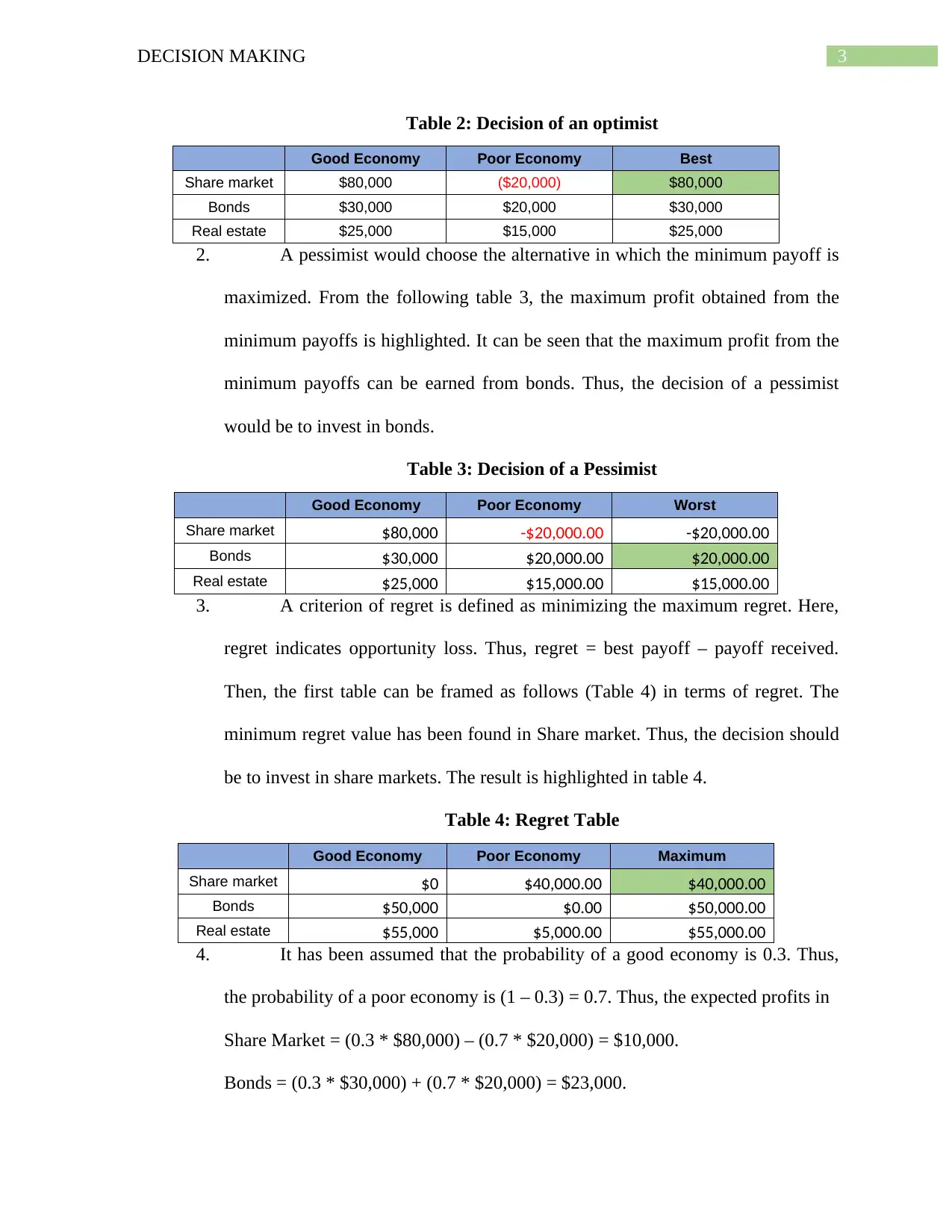
Table 2: Decision of an optimist
Good Economy Poor Economy Best
Share market $80,000 ($20,000) $80,000
Bonds $30,000 $20,000 $30,000
Real estate $25,000 $15,000 $25,000
2. A pessimist would choose the alternative in which the minimum payoff is
maximized. From the following table 3, the maximum profit obtained from the
minimum payoffs is highlighted. It can be seen that the maximum profit from the
minimum payoffs can be earned from bonds. Thus, the decision of a pessimist
would be to invest in bonds.
Table 3: Decision of a Pessimist
Good Economy Poor Economy Worst
Share market $80,000 -$20,000.00 -$20,000.00
Bonds $30,000 $20,000.00 $20,000.00
Real estate $25,000 $15,000.00 $15,000.00
3. A criterion of regret is defined as minimizing the maximum regret. Here,
regret indicates opportunity loss. Thus, regret = best payoff – payoff received.
Then, the first table can be framed as follows (Table 4) in terms of regret. The
minimum regret value has been found in Share market. Thus, the decision should
be to invest in share markets. The result is highlighted in table 4.
Table 4: Regret Table
Good Economy Poor Economy Maximum
Share market $0 $40,000.00 $40,000.00
Bonds $50,000 $0.00 $50,000.00
Real estate $55,000 $5,000.00 $55,000.00
4. It has been assumed that the probability of a good economy is 0.3. Thus,
the probability of a poor economy is (1 – 0.3) = 0.7. Thus, the expected profits in
Share Market = (0.3 * $80,000) – (0.7 * $20,000) = $10,000.
Bonds = (0.3 * $30,000) + (0.7 * $20,000) = $23,000.

4DECISION MAKING
Real Estate = (0.3 * $25,000) – (0.7 * $15,000) = $18,000.
Thus, the optimal action will be to invest in Bonds according to the
assumption in this question.
5. The expected value of perfect information (EVPI) is given by the formula
EVPI=∑
j
p j ( max
i Rij )−max
i ∑
j
p j Rij, where, Rij is the value of the ith row and jth
column and pj is the probability of that cell.
Thus, ∑
j
p j (max
i Rij ) = (0.3 * $80,000) + (0.3 * $30,000) + (0.3 * $25,000) =
$40,500.
Again, max
i ∑
j
p j Rij=¿$23,000.
Therefore, EVPI = $(40,500 – 23000) = $17,500.

5DECISION MAKING
ANSWER 2
(a) Jerry wants to open a bicycle shop. He can open two types of shops – large shops
(a1) and small shops (a2). There are two types of markets – good market (s1) and poor
market (s2). According to his beliefs, in a large shop, there will be a profit of $80,000 in a
good market and a loss of $40,000 in a poor market. There is a 50 percent chance for the
market to be good or bad. Thus, in a large shop, the estimated profit will be:
P (a1) = $80,000 * P (s1) + $(- 40,000) * P (s2)
= $(80,000 * 0.5 – 40,000 * 0.5)
= $20,000.
In a small shop, jerry believes that there will be a profit of $30,000 in a good
market and a loss of $10,000 in a poor market. Thus, in a small shop, the estimated profit
will be:
P (a2) = $30,000 * P (s1) + $(- 10,000) * P (s2)
= $(30,000 * 0.5 – 10,000 * 0.5)
= $10,000.
Thus, whether the market is good or bad, profit is more in a large shop compared
to a small shop. Thus, Jerry should open a large shop.
(b) Considering the track record provided by Jerry’s friend, the prior probabilities has
been revised. Here a favorable market has been considered as X and an unfavorable
market has been considered as Y. Irrespective of good or poor market conditions, in an
unfavorable market, there has been no profit or loss. Thus, in a large shop, the revised
prior probability will be:
P (a1) = P (s1) * P (X) + P (s2) * P (Y)

6DECISION MAKING
= 0.5 * 0.8 + 0.5 * 0.2
= 0.5.
Thus, in a small shop, the revised prior probability will be:
P (a2) = P (s1) * P (X) + P (s2) * P (Y)
= 0.5 * 0.8 + 0.5 * 0.4
= 0.5.
(c) The posterior probability of a good market given that his friend has provided an
unfavorable market prediction is P (s1) * P (Y) = 0.5 * 0.2 = 0.1.
(d) The expected net gain in a large market is
P (a1) = $80,000 * P (s1) * P (X) + $(- 40,000) * P (s2) * P (Y)
= $(80,000 * 0.5 * 0.8 – 40,000 * 0.5 * 0.2)
= $24,000.
The expected gain in small market is
P (a2) = $30,000 * P (s1) * P (X) + $(- 10,000) * P (s2) * P (Y)
= $(30,000 * 0.5 * 0.8 – 10,000 * 0.5 * 0.2)
= $10,000.
If his friend is engaged to conduct the market research, the profit in the large
market will become $(24,000 – 3,000) = $21,000 and in the small market will become
$(10,000 – 3,000) = $7,000.
Thus, if his friend is engaged, his profit in the large market will increase and his
profit in the small market will decrease. Thus, there is not much increase in the profits by
engaging his friend and conducting the market research. Hence, his friend should not be
involved.

7DECISION MAKING
ANSWER 3
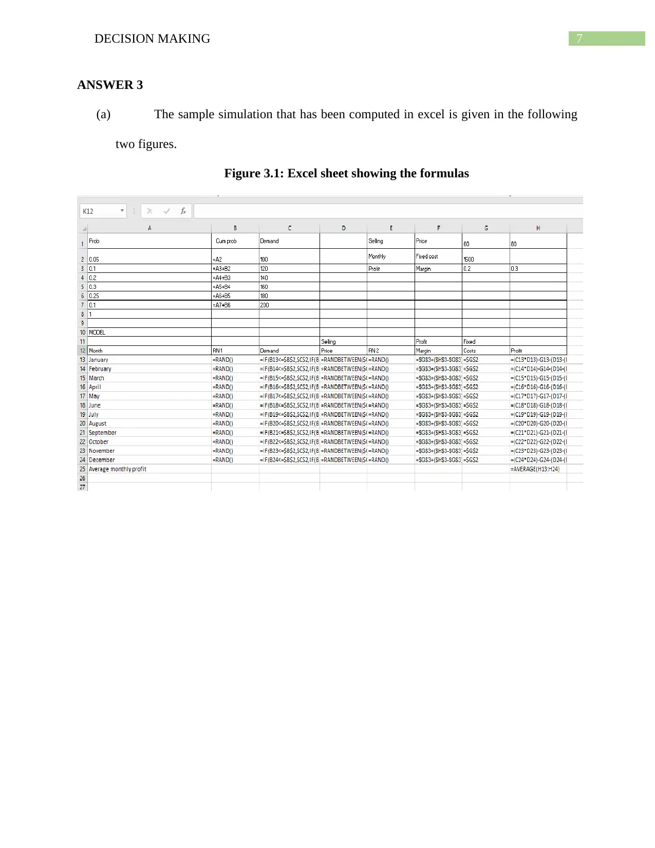
(a) The sample simulation that has been computed in excel is given in the following
two figures.
Figure 3.1: Excel sheet showing the formulas

8DECISION MAKING
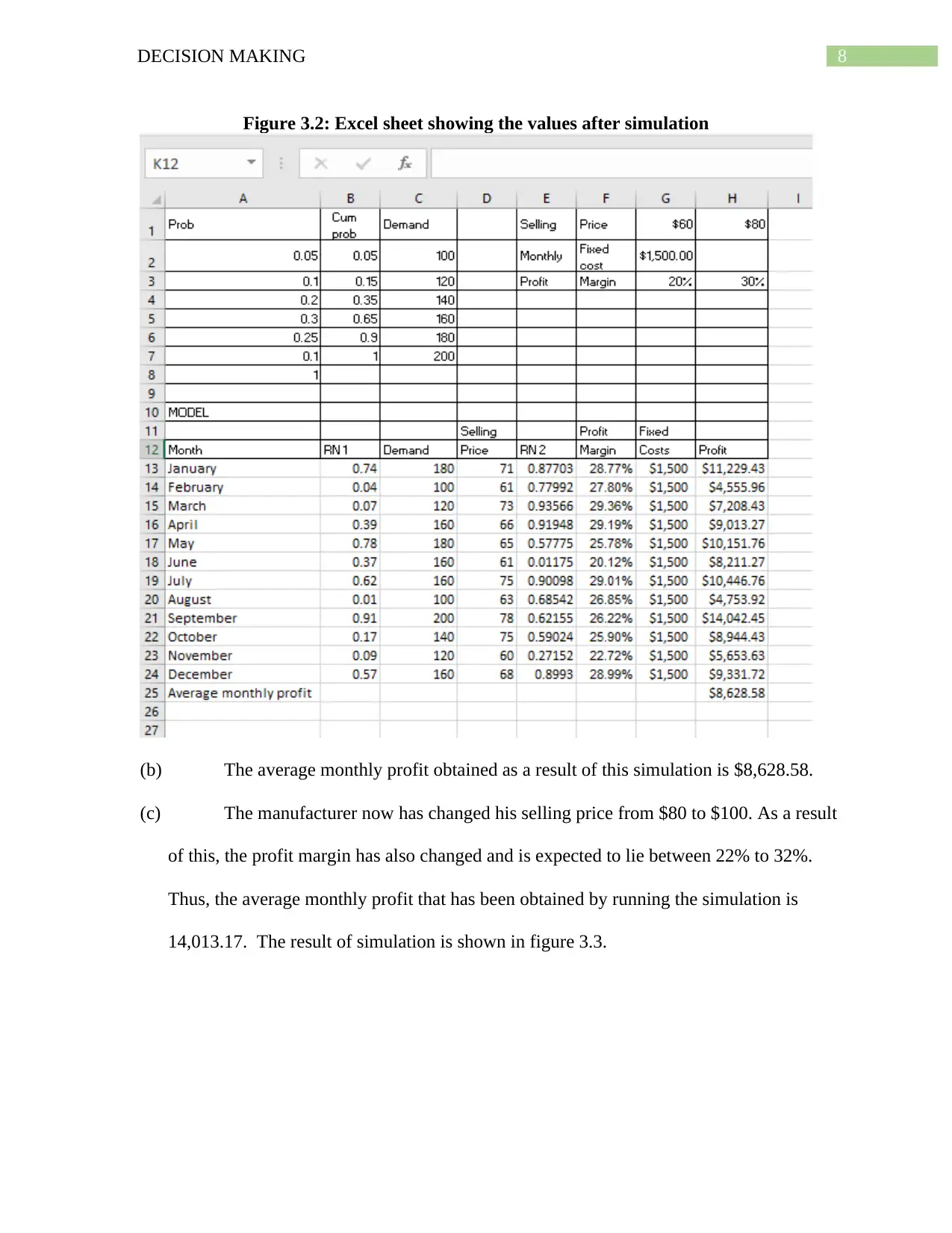
Figure 3.2: Excel sheet showing the values after simulation
(b) The average monthly profit obtained as a result of this simulation is $8,628.58.
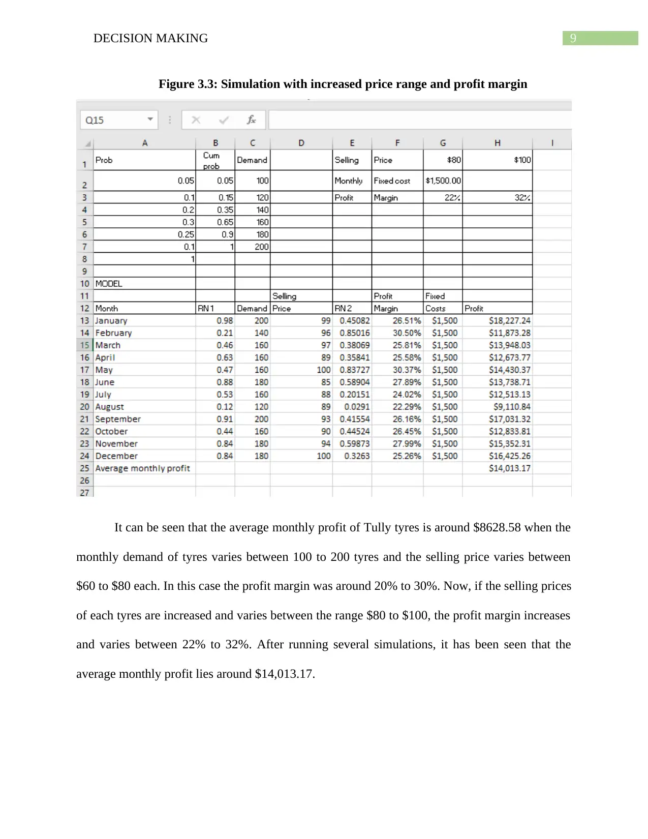
(c) The manufacturer now has changed his selling price from $80 to $100. As a result
of this, the profit margin has also changed and is expected to lie between 22% to 32%.
Thus, the average monthly profit that has been obtained by running the simulation is
14,013.17. The result of simulation is shown in figure 3.3.

9DECISION MAKING
Figure 3.3: Simulation with increased price range and profit margin
It can be seen that the average monthly profit of Tully tyres is around $8628.58 when the
monthly demand of tyres varies between 100 to 200 tyres and the selling price varies between
$60 to $80 each. In this case the profit margin was around 20% to 30%. Now, if the selling prices
of each tyres are increased and varies between the range $80 to $100, the profit margin increases
and varies between 22% to 32%. After running several simulations, it has been seen that the
average monthly profit lies around $14,013.17.

10DECISION MAKING
ANSWER 4
(a) The table that is necessary to estimate the overhead cost using the high-low
method is given as follows:
Table 4.1: High-Low Method
Machine Hours (x) Overhead Cost (y)
Highest Activity 3800 $48,000
Lowest Activity 1800 $46,000
Therefore, the variable cost per unit is $ (48,000−46,000)
3800−1800 =1.
The total fixed cost is $(48,000 – 1 * 3800) = $(46,000 – 1 * 1800) = $44,200.
Thus, the overhead cost can be estimated by the equation: y = 44,200 + 1 * x.
Thus, when 3000 machine hours were used, the overhead cost can be estimated as
$(44,200 + 3,000) = $47,200.
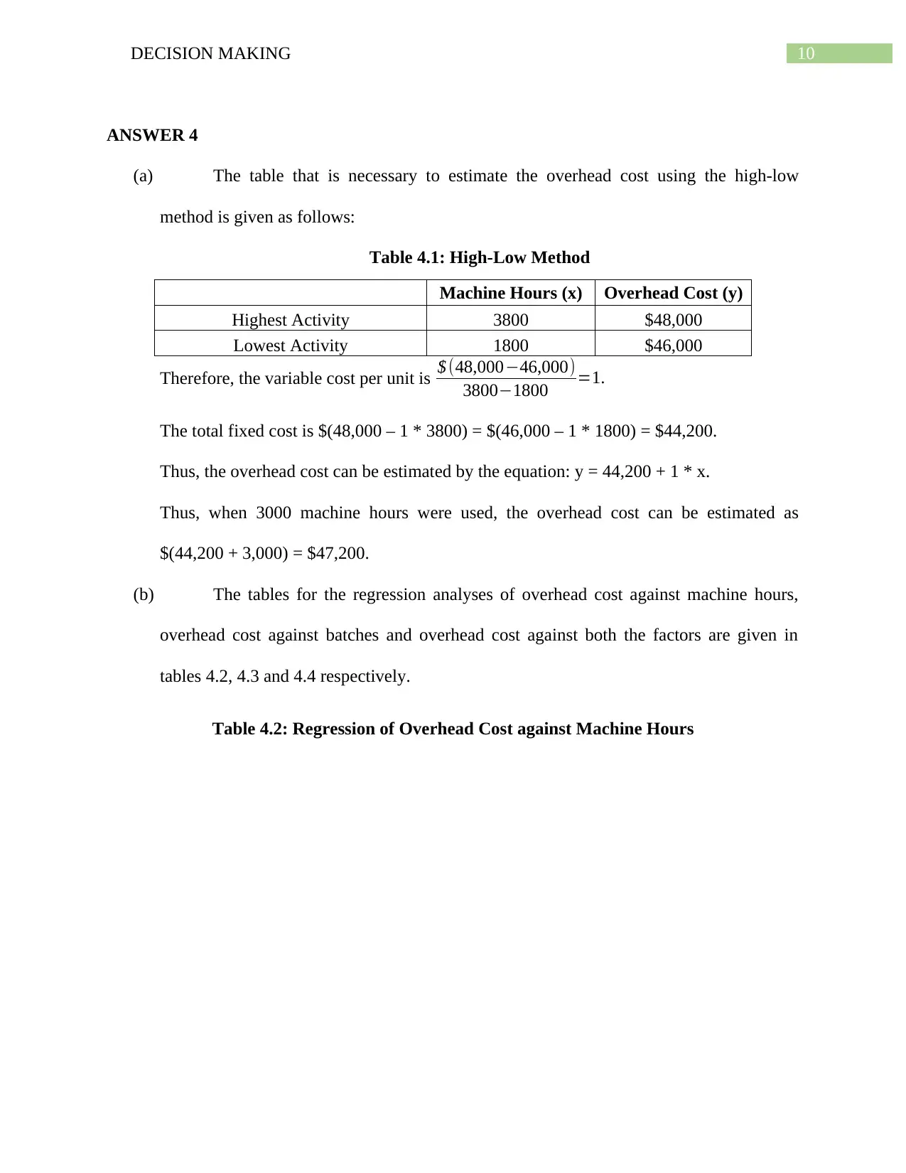
(b) The tables for the regression analyses of overhead cost against machine hours,
overhead cost against batches and overhead cost against both the factors are given in
tables 4.2, 4.3 and 4.4 respectively.
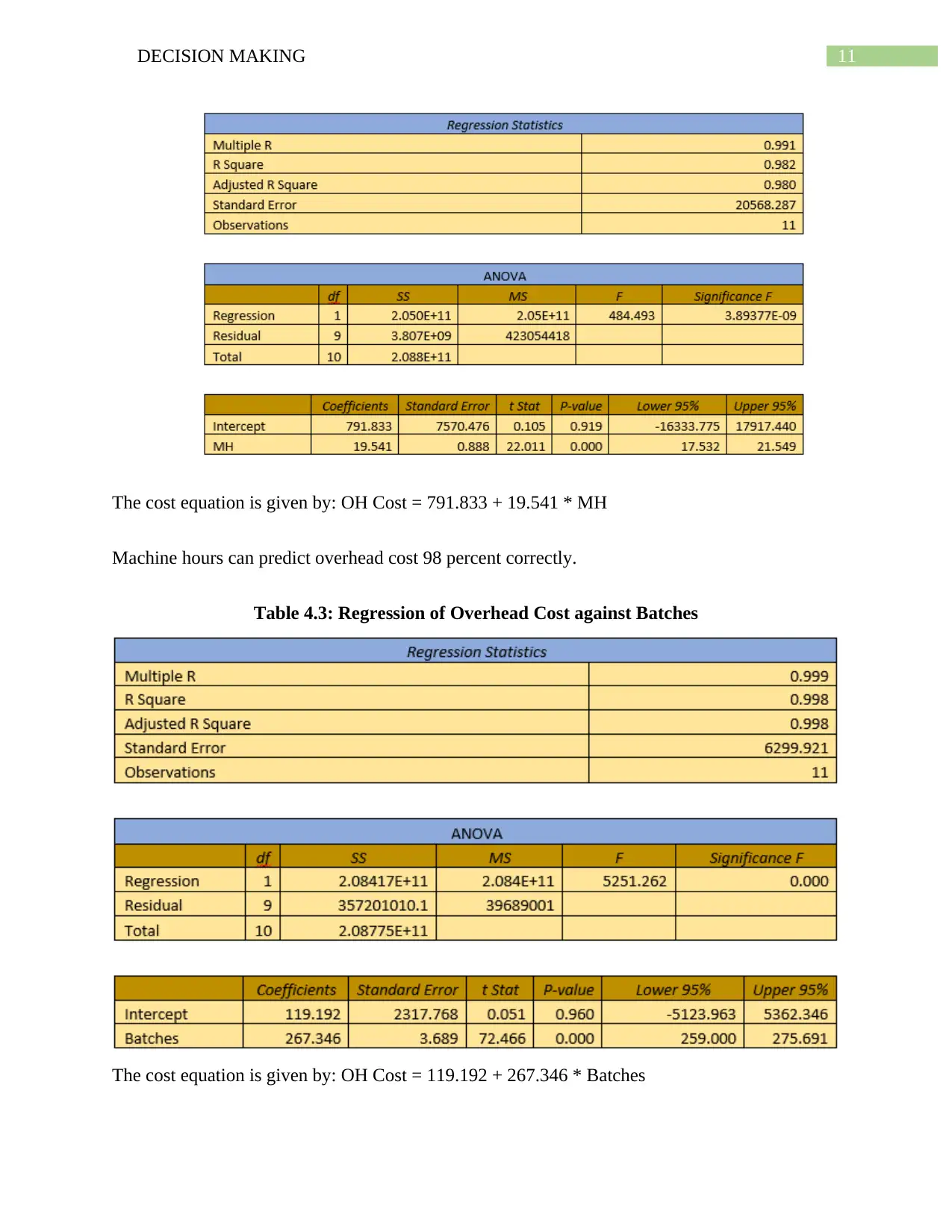
Table 4.2: Regression of Overhead Cost against Machine Hours

11DECISION MAKING
The cost equation is given by: OH Cost = 791.833 + 19.541 * MH
Machine hours can predict overhead cost 98 percent correctly.
Table 4.3: Regression of Overhead Cost against Batches
The cost equation is given by: OH Cost = 119.192 + 267.346 * Batches