Production and Cost Analysis Case Study for ECO 520 Course

This case study examines the production and cost functions of firms in a perfectly competitive market, employing a Cobb-Douglas production function. The analysis begins with deriving production and cost functions, including calculations of total, fixed, and variable costs. It then explores isoquants and the relationship between labor and capital. The study progresses to analyze short-run and long-run equilibrium, incorporating graphical representations of supply and demand curves. The case study determines the optimal output, revenue, cost, and profit for a firm, illustrating short-run equilibrium in a competitive market. Furthermore, the analysis extends to long-run equilibrium, examining the impact of new firms entering the market due to positive profits. Finally, the study calculates the average and marginal costs in the long run, concluding with the determination of the long-run equilibrium output for each firm and the industry output, considering the number of firms in the market. The study uses algebraic derivations, graphical representations, and numerical computations to provide a comprehensive understanding of microeconomic principles in a competitive market setting.

Running head: CASE STUDY ON PRODUCTION AND COST
Case Study on Production and Cost
Name of the Student:
Name of the University:
Author Note:

1
CASE STUDY ON PRODUCTION AND COST
Table of Contents
Answer 1....................................................................................................................................3
Answer 1.1.............................................................................................................................3
Answer 1.2.............................................................................................................................3
Answer 2....................................................................................................................................3
Answer 2.1.............................................................................................................................3
Answer 2.2.............................................................................................................................4
Answer 2.3.............................................................................................................................4
Answer 3....................................................................................................................................4
Answer 3.1.............................................................................................................................4
Answer 3.2.............................................................................................................................5
Answer 3.3.............................................................................................................................5
Answer 3.4.............................................................................................................................6
Answer 4....................................................................................................................................7
Answer 4.1.............................................................................................................................7
Answer 5....................................................................................................................................7
Answer 5.1.............................................................................................................................7
Answer 6....................................................................................................................................8
Answer 6.1.............................................................................................................................8
Answer 7....................................................................................................................................8
Answer 8....................................................................................................................................9
Answer 8..................................................................................................................................10

2
CASE STUDY ON PRODUCTION AND COST
Reference..................................................................................................................................11

3
CASE STUDY ON PRODUCTION AND COST
Answer 1
Answer 1.1
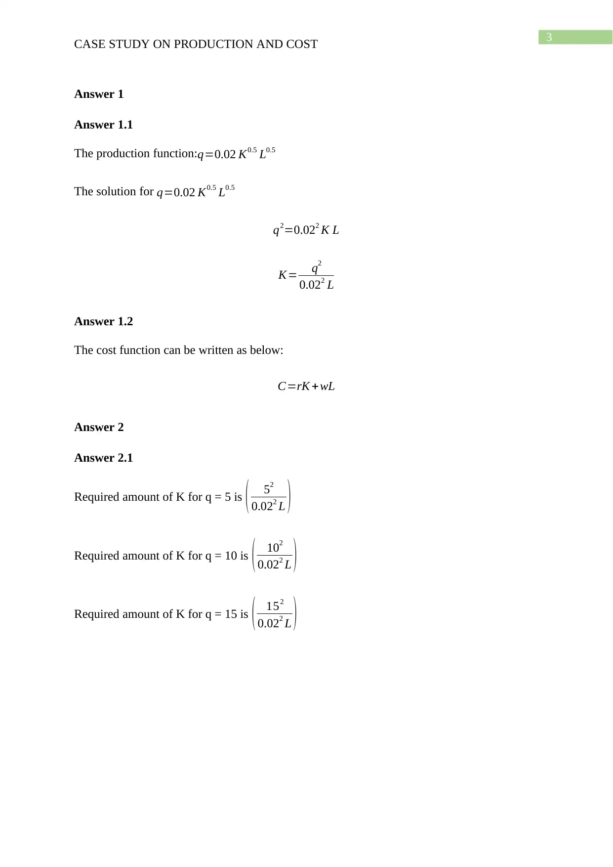
The production function:q=0.02 K0.5 L0.5
The solution for q=0.02 K0.5 L0.5
q2=0.022 K L
K= q2
0.022 L
Answer 1.2
The cost function can be written as below:
C=rK +wL
Answer 2
Answer 2.1
Required amount of K for q = 5 is ( 52
0.022 L )
Required amount of K for q = 10 is ( 102
0.022 L )
Required amount of K for q = 15 is ( 152
0.022 L )

4
CASE STUDY ON PRODUCTION AND COST
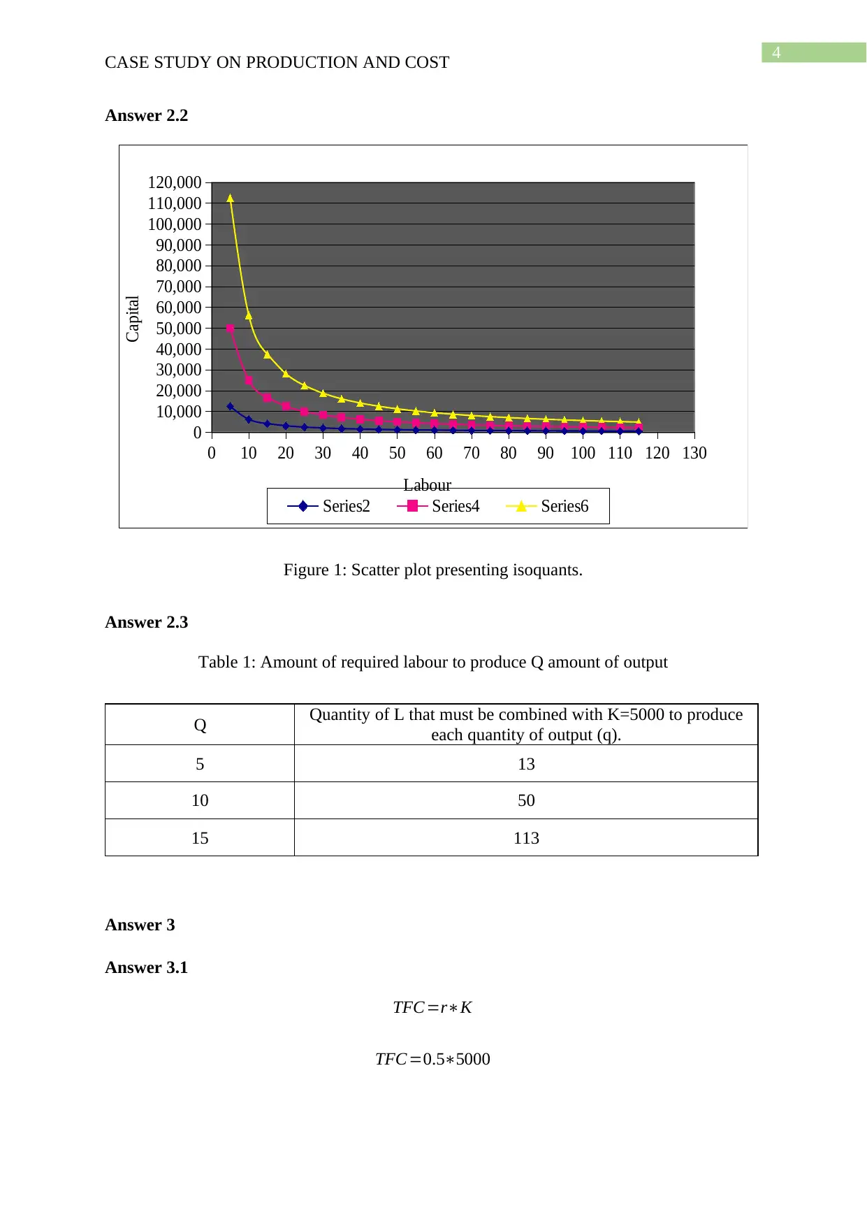
Answer 2.2
0 10 20 30 40 50 60 70 80 90 100 110 120 130
0
10,000
20,000
30,000
40,000
50,000
60,000
70,000
80,000
90,000
100,000
110,000
120,000
Series2 Series4 Series6
Labour
Capital
Figure 1: Scatter plot presenting isoquants.
Answer 2.3
Table 1: Amount of required labour to produce Q amount of output
Q Quantity of L that must be combined with K=5000 to produce
each quantity of output (q).
5 13
10 50
15 113
Answer 3
Answer 3.1
TFC =r∗K
TFC =0.5∗5000

5
CASE STUDY ON PRODUCTION AND COST
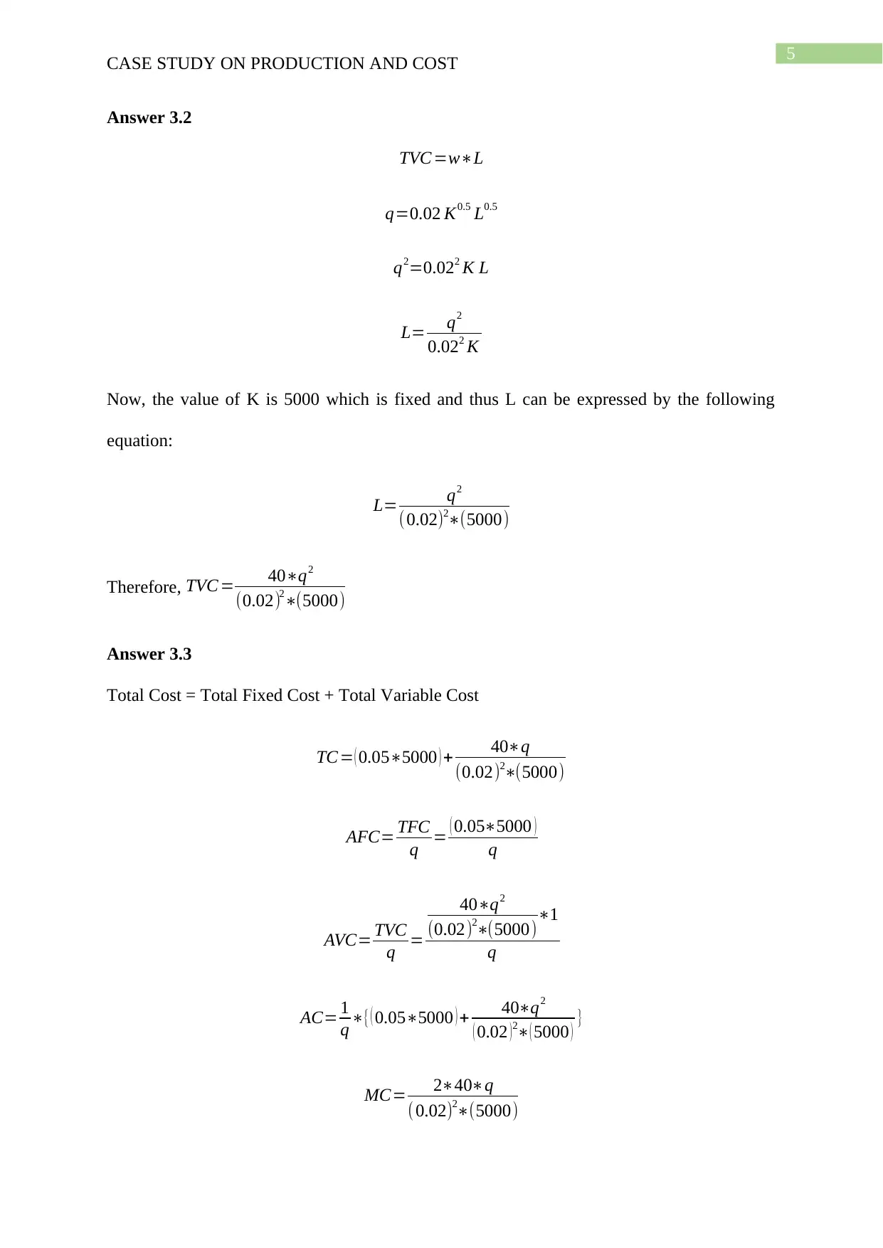
Answer 3.2
TVC =w∗L
q=0.02 K0.5 L0.5
q2=0.022 K L
L= q2
0.022 K
Now, the value of K is 5000 which is fixed and thus L can be expressed by the following
equation:
L= q2
(0.02)2∗(5000)
Therefore, TVC = 40∗q2
(0.02)2∗(5000)
Answer 3.3
Total Cost = Total Fixed Cost + Total Variable Cost
TC= ( 0.05∗5000 ) + 40∗q
(0.02)2∗(5000)
AFC= TFC
q = ( 0.05∗5000 )
q
AVC= TVC
q =
40∗q2
(0.02)2∗(5000)∗1
q
AC= 1
q ∗{( 0.05∗5000 ) + 40∗q2
( 0.02 ) 2∗( 5000 ) }
MC= 2∗40∗q
( 0.02)2∗(5000)

6
CASE STUDY ON PRODUCTION AND COST
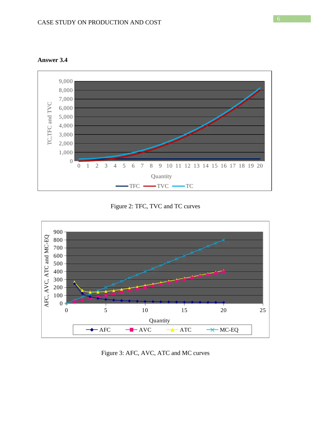
Answer 3.4
0 1 2 3 4 5 6 7 8 9 10 11 12 13 14 15 16 17 18 19 20
0
1,000
2,000
3,000
4,000
5,000
6,000
7,000
8,000
9,000
TFC TVC TC
Quantity
TC,TFC and TVC
Figure 2: TFC, TVC and TC curves
0 5 10 15 20 25
0
100
200
300
400
500
600
700
800
900
AFC AVC ATC MC-EQ
Quantity
AFC, AVC, ATC and MC-EQ
Figure 3: AFC, AVC, ATC and MC curves

7
CASE STUDY ON PRODUCTION AND COST
Answer 4
Answer 4.1
0
100
200
300
400
500
600
700
800
900
1000
1100
1200
1300
1400
1500
1600
1700
1800
1900
2000
-300
-200
-100
0
100
200
300
400
500
600
700
800
900
Demand Supply
Market Quantity
Price
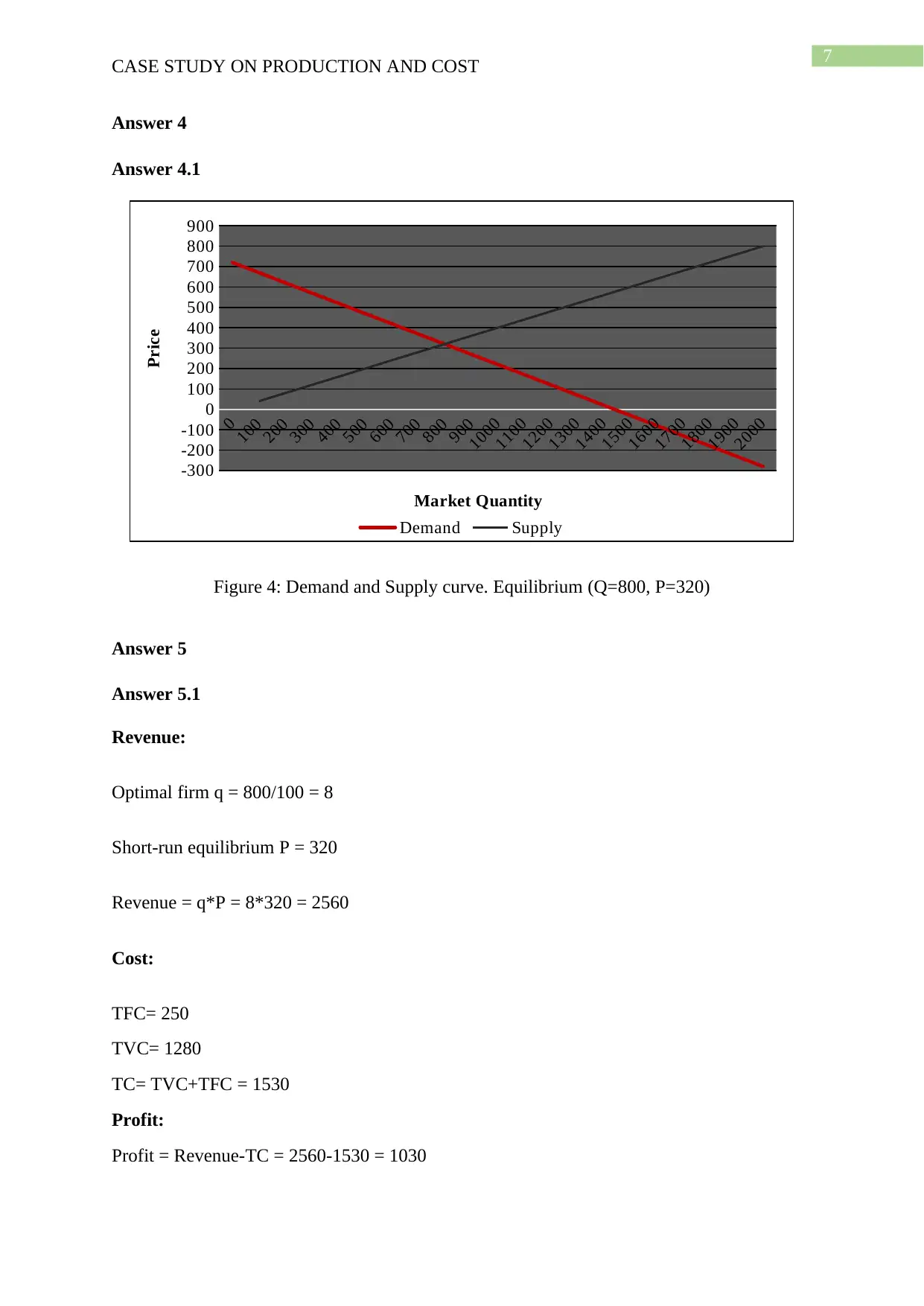
Figure 4: Demand and Supply curve. Equilibrium (Q=800, P=320)
Answer 5
Answer 5.1
Revenue:
Optimal firm q = 800/100 = 8
Short-run equilibrium P = 320
Revenue = q*P = 8*320 = 2560
Cost:
TFC= 250
TVC= 1280
TC= TVC+TFC = 1530
Profit:
Profit = Revenue-TC = 2560-1530 = 1030

8
CASE STUDY ON PRODUCTION AND COST
Answer 6
Answer 6.1
0 1 2 3 4 5 6 7 8 9 10 11 12 13 14 15 16 17 18 19 20
0
100
200
300
400
500
600
700
800
900
AVC ATC MC-EQ P
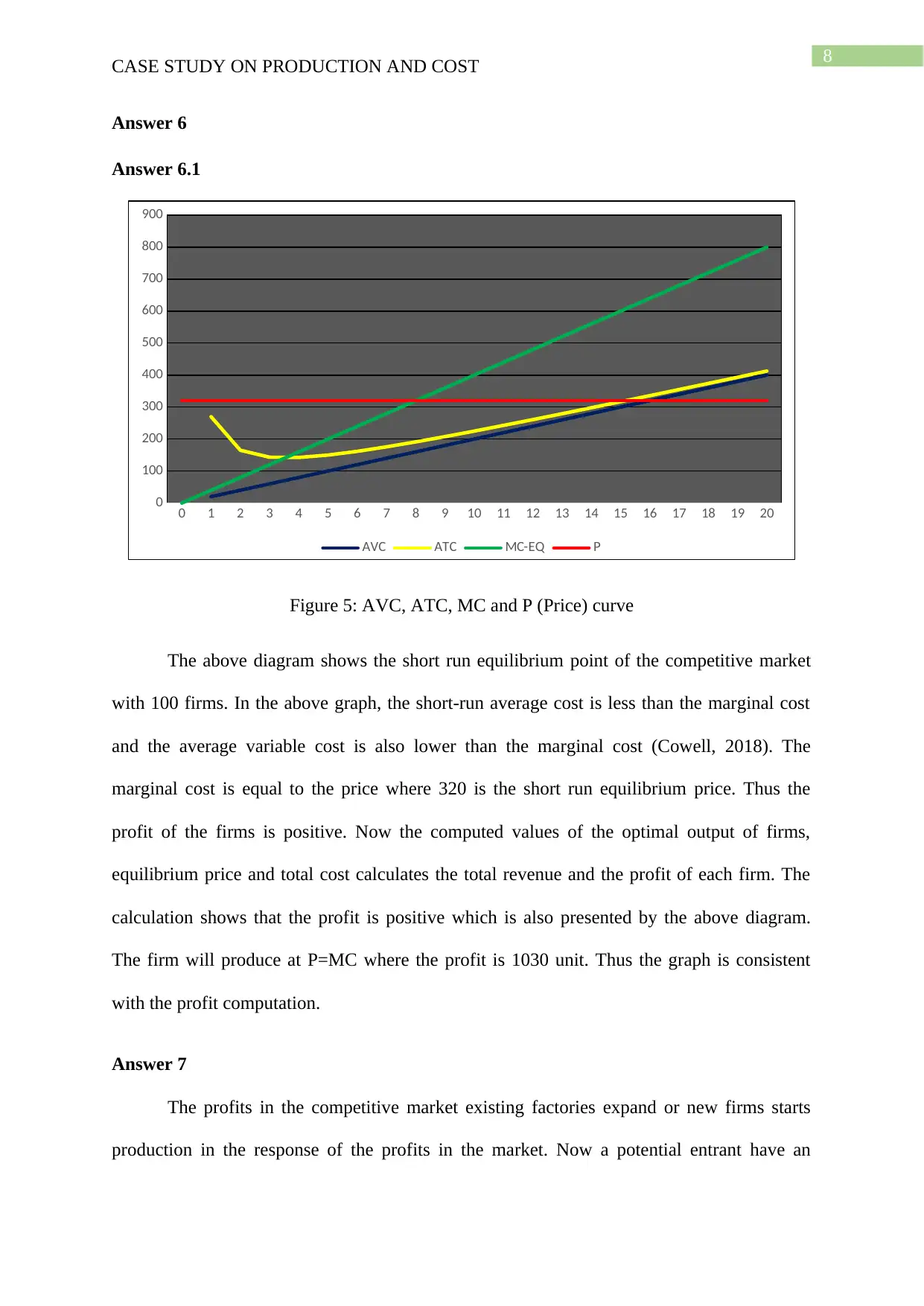
Figure 5: AVC, ATC, MC and P (Price) curve
The above diagram shows the short run equilibrium point of the competitive market
with 100 firms. In the above graph, the short-run average cost is less than the marginal cost
and the average variable cost is also lower than the marginal cost (Cowell, 2018). The
marginal cost is equal to the price where 320 is the short run equilibrium price. Thus the
profit of the firms is positive. Now the computed values of the optimal output of firms,
equilibrium price and total cost calculates the total revenue and the profit of each firm. The
calculation shows that the profit is positive which is also presented by the above diagram.
The firm will produce at P=MC where the profit is 1030 unit. Thus the graph is consistent
with the profit computation.
Answer 7
The profits in the competitive market existing factories expand or new firms starts
production in the response of the profits in the market. Now a potential entrant have an

9
CASE STUDY ON PRODUCTION AND COST
exactly identical cost function which means the cost the new firm have to bare is equal to the
cost of production for the existing firms. Now, the profit of the existing firms is positive
which indicates that the potential entrants will earn profit if they enter in the market (Lewis &
Stevens, 2015). So, the identical cost function of the entrant and the positive profit of the
existing firms encourages the potential entrant to enter the market and the entrant will enter in
the market.
Answer 8
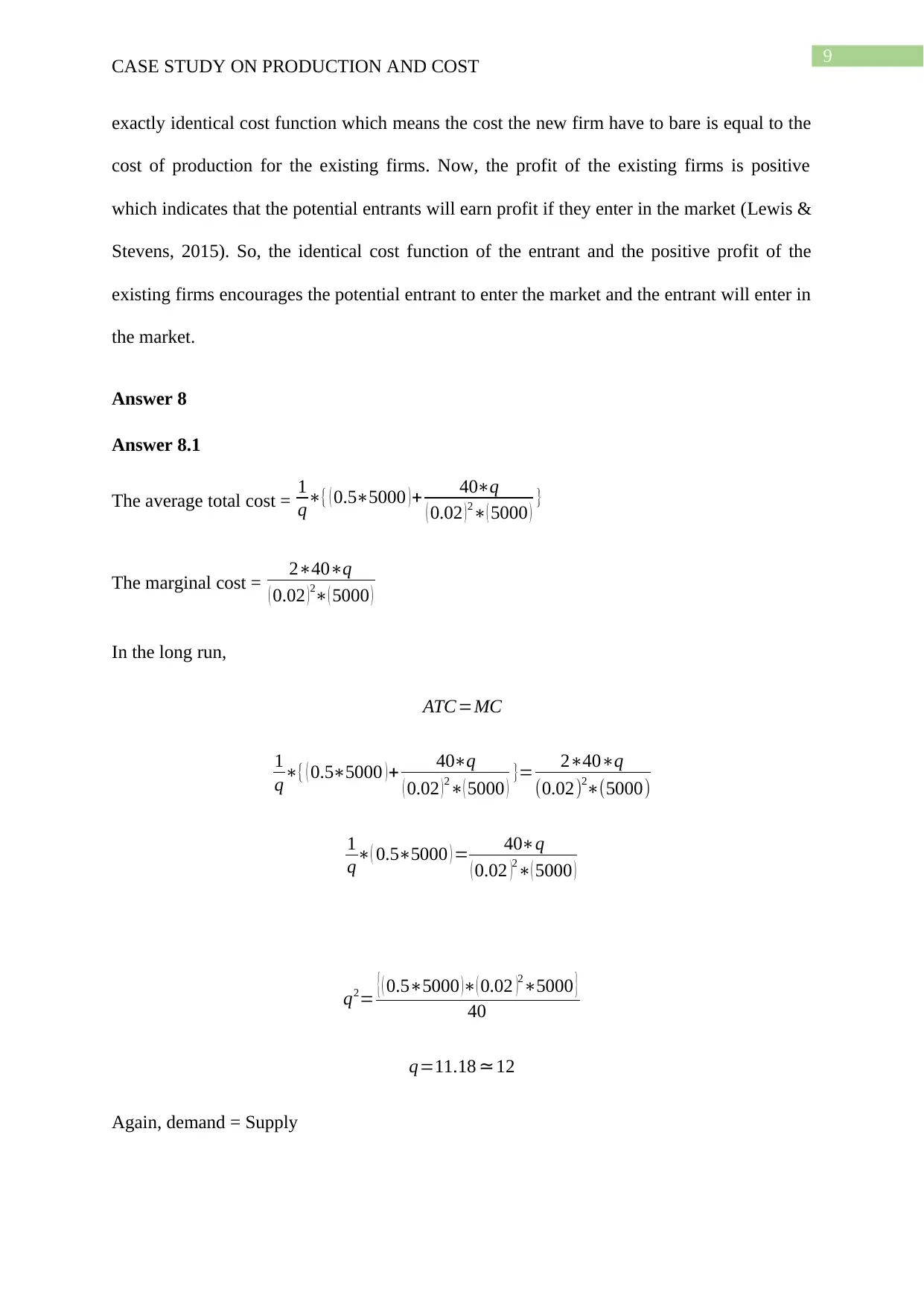
Answer 8.1
The average total cost = 1
q∗{ ( 0.5∗5000 )+ 40∗q
( 0.02 )2∗( 5000 ) }
The marginal cost = 2∗40∗q
( 0.02 ) 2∗( 5000 )
In the long run,
ATC=MC
1
q∗{ ( 0.5∗5000 )+ 40∗q
( 0.02 )2∗( 5000 ) }= 2∗40∗q
(0.02)2∗(5000)
1
q∗( 0.5∗5000 ) = 40∗q
( 0.02 )2∗( 5000 )
q2= { ( 0.5∗5000 )∗( 0.02 )2∗5000 }
40
q=11.18 ≃12
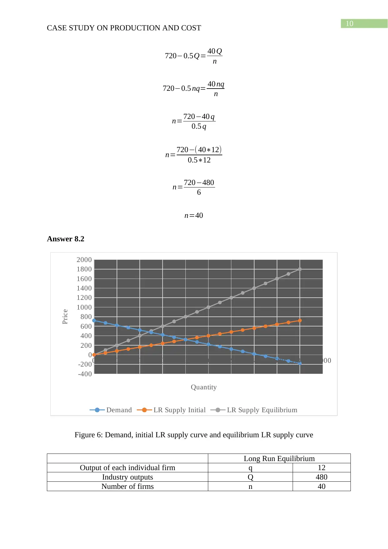
Again, demand = Supply

10
CASE STUDY ON PRODUCTION AND COST
720−0.5Q= 40 Q
n
720−0.5 nq= 40 nq
n
n=720−40 q
0.5 q
n=720−( 40∗12)
0.5∗12
n=720−480
6
n=40
Answer 8.2
0 200 400 600 800 1,000 1,200 1,400 1,600 1,800 2,000
-400
-200
0
200
400
600
800
1000
1200
1400
1600
1800
2000
Demand LR Supply Initial LR Supply Equilibrium
Quantity
Price
Figure 6: Demand, initial LR supply curve and equilibrium LR supply curve
Long Run Equilibrium
Output of each individual firm q 12
Industry outputs Q 480
Number of firms n 40

11
CASE STUDY ON PRODUCTION AND COST