PSCY 2211 Statistics Homework: Hypothesis Testing and SPSS Analysis
VerifiedAdded on 2023/04/21
|17
|3416
|65
Homework Assignment
AI Summary
This assignment provides solutions to several statistics problems involving hypothesis testing. It covers ANOVA tests to determine the effect of breakfast drinks on test performance and the impact of cellphone designs on text talk. Additionally, it examines the effect of caffeine levels on energy. Chi-Square tests are used to analyze the association between political party and gender, as well as the relationship between party food choices and alcohol consumption. Finally, regression analysis is employed to assess the influence of IQ and class engagement on students' final grades. The solutions include detailed interpretations of SPSS outputs, p-values, and post-hoc analyses, offering a comprehensive understanding of the statistical methods applied. Desklib offers a wide range of solved assignments and past papers for students seeking academic assistance.
Statistics
Student Name:
Instructor Name:
Course Number:
29 March 2019
Student Name:
Instructor Name:
Course Number:
29 March 2019
Paraphrase This Document
Need a fresh take? Get an instant paraphrase of this document with our AI Paraphraser
Question 2:
For this question, we sought to test whether there breakfast drink differentially affect test
performance. A researcher randomly assigns participants to five different ‘drink groups: Coffee,
Tea, Orange Juice, Apple Juice, or Water. Each participant drinks their designated fluid for
breakfast and then engages in a statistics exam. Higher scores on the exam indicate greater
performance. The following data was collected:
Table 1: Data
Coffee Tea Orange Juice Apple Juice Water
4 6 5 7 7
11 6 3 8 7
11 13 13 10 11
23 12 10 19 11
11 14 15 11 11
To test this, the following hypothesis was developed.
Null hypothesis (H0): There is no significant difference in the test performance based on the type
of breakfast drink taken.
Alternative hypothesis (HA): There is significant difference in the test performance based on the
type of breakfast drink taken.
Analysis of variance (ANOVA) test was performed and results compared at 5% level of
significance. Results are presented below;
Table 2: ANOVA
Sum of Squares df Mean Square F Sig.
Between Groups 26.960 4 6.740 .291 .880
Within Groups 462.800 20 23.140
Total 489.760 24
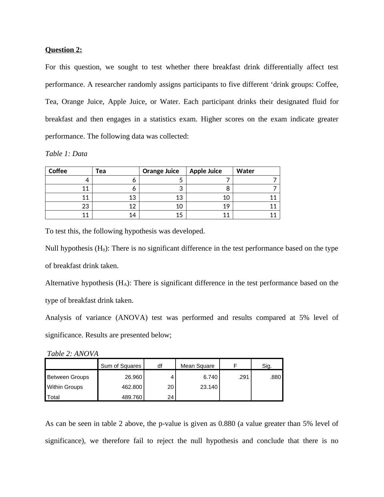
As can be seen in table 2 above, the p-value is given as 0.880 (a value greater than 5% level of
significance), we therefore fail to reject the null hypothesis and conclude that there is no
For this question, we sought to test whether there breakfast drink differentially affect test
performance. A researcher randomly assigns participants to five different ‘drink groups: Coffee,
Tea, Orange Juice, Apple Juice, or Water. Each participant drinks their designated fluid for
breakfast and then engages in a statistics exam. Higher scores on the exam indicate greater
performance. The following data was collected:
Table 1: Data
Coffee Tea Orange Juice Apple Juice Water
4 6 5 7 7
11 6 3 8 7
11 13 13 10 11
23 12 10 19 11
11 14 15 11 11
To test this, the following hypothesis was developed.
Null hypothesis (H0): There is no significant difference in the test performance based on the type
of breakfast drink taken.
Alternative hypothesis (HA): There is significant difference in the test performance based on the
type of breakfast drink taken.
Analysis of variance (ANOVA) test was performed and results compared at 5% level of
significance. Results are presented below;
Table 2: ANOVA
Sum of Squares df Mean Square F Sig.
Between Groups 26.960 4 6.740 .291 .880
Within Groups 462.800 20 23.140
Total 489.760 24
As can be seen in table 2 above, the p-value is given as 0.880 (a value greater than 5% level of
significance), we therefore fail to reject the null hypothesis and conclude that there is no
significant difference in the test performance based on the type of breakfast drink taken. That is,
breakfast drink does not differentially affect test performance.
Question 3:
For this question, an investigator conducts an experiment to assess the effect of cellphone
designs on ‘text talk’ (e.g., using k instead of okay, using idk instead of I don’t know). Three
samples of individuals were given material to type on a particular cellphone type (a, b, or c), and
the number of text talk uses by each participant was recorded (Anscombe, 2015). Higher scores
indicate more text talk usage. The data are as follows:
Table 3: Data
A B C
0 6 6
4 8 5
0 5 9
1 4 4
0 2 6
⊘ This is a preview!⊘
Do you want full access?
Subscribe today to unlock all pages.
Trusted by 1+ million students worldwide
To test this, the following hypothesis was developed.
Null hypothesis (H0): There is no significant difference in the number of text talk based on the
type cellphone.
Alternative hypothesis (HA): There is significant difference in the number of text talk based on
the type cellphone.
Analysis of variance (ANOVA) test was performed and results compared at 5% level of
significance. Results are presented below;
Table 4: Descriptive
N Mean Std. Deviation Std. Error 95% Confidence Interval for Mean
Lower Bound Upper Bound
A 5 1.0000 1.73205 .77460 -1.1506 3.1506
B 5 5.0000 2.23607 1.00000 2.2236 7.7764
C 5 6.0000 1.87083 .83666 3.6771 8.3229
Total 15 4.0000 2.87849 .74322 2.4059 5.5941
Table 5: ANOVA
Sum of Squares df Mean Square F Sig.
Between Groups 70.000 2 35.000 9.130 .004
Within Groups 46.000 12 3.833
Total 116.000 14
As can be seen in table 5 above, the p-value is given as 0.004 (a value less than 5% level of
significance), we therefore reject the null hypothesis and conclude that there is significant
difference in the number of text talk based on the type cellphone. That is, the type of cellphone
design affects the text talk (Nikolić, Muresan, Feng, & Singer, 2012).
Table 6: Multiple Comparisons
(I) Type of
cellphone
(J) Type of
cellphone
Mean
Difference (I-J)
Std. Error Sig. 95% Confidence Interval
Lower Bound Upper Bound
A B -4.00000* 1.23828 .022 -7.4418 -.5582
C -5.00000* 1.23828 .005 -8.4418 -1.5582
Paraphrase This Document
Need a fresh take? Get an instant paraphrase of this document with our AI Paraphraser
B A 4.00000* 1.23828 .022 .5582 7.4418
C -1.00000 1.23828 1.000 -4.4418 2.4418
C A 5.00000* 1.23828 .005 1.5582 8.4418
B 1.00000 1.23828 1.000 -2.4418 4.4418
*. The mean difference is significant at the 0.05 level.
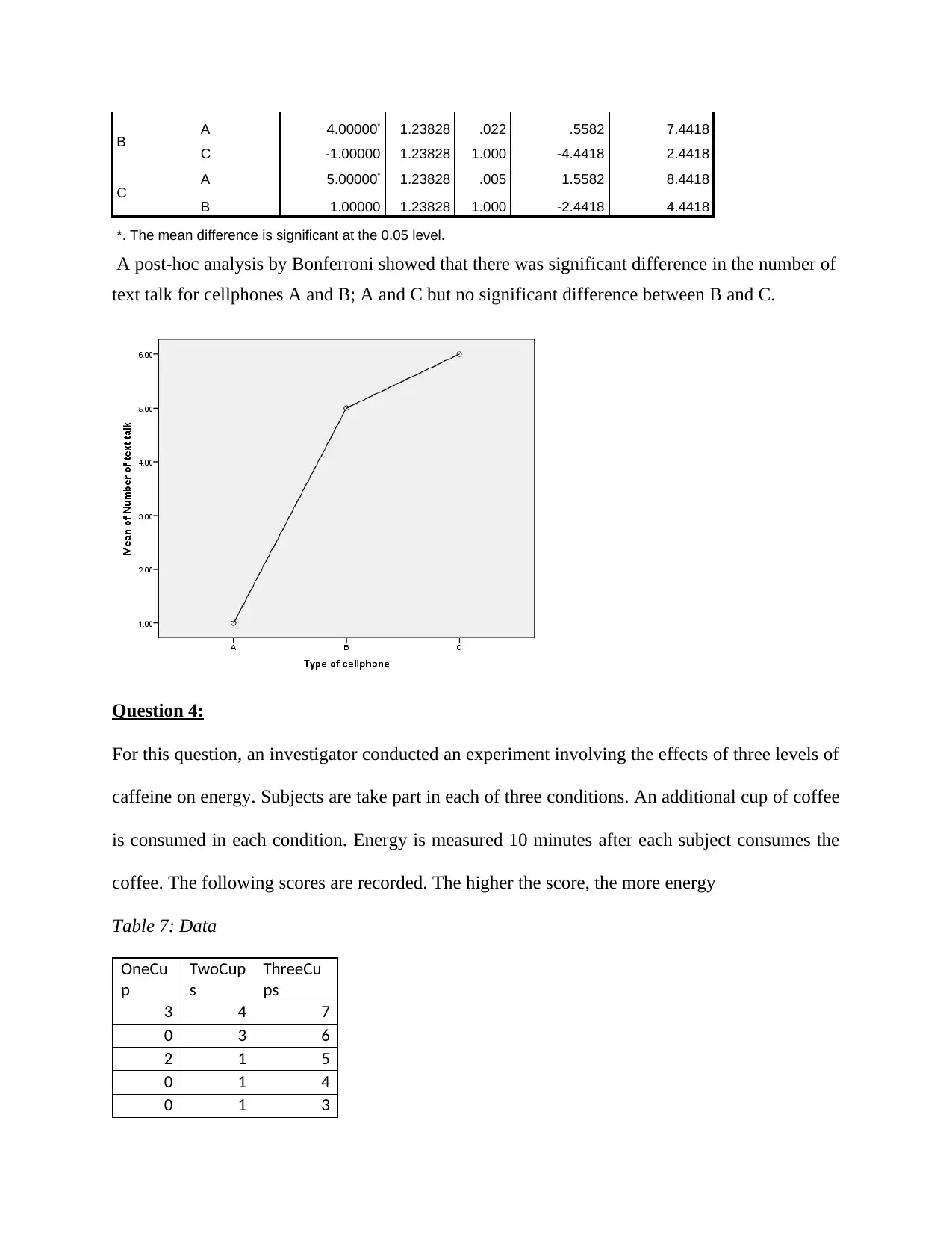
A post-hoc analysis by Bonferroni showed that there was significant difference in the number of
text talk for cellphones A and B; A and C but no significant difference between B and C.
Question 4:
For this question, an investigator conducted an experiment involving the effects of three levels of
caffeine on energy. Subjects are take part in each of three conditions. An additional cup of coffee
is consumed in each condition. Energy is measured 10 minutes after each subject consumes the
coffee. The following scores are recorded. The higher the score, the more energy
Table 7: Data
OneCu
p
TwoCup
s
ThreeCu
ps
3 4 7
0 3 6
2 1 5
0 1 4
0 1 3
C -1.00000 1.23828 1.000 -4.4418 2.4418
C A 5.00000* 1.23828 .005 1.5582 8.4418
B 1.00000 1.23828 1.000 -2.4418 4.4418
*. The mean difference is significant at the 0.05 level.
A post-hoc analysis by Bonferroni showed that there was significant difference in the number of
text talk for cellphones A and B; A and C but no significant difference between B and C.
Question 4:
For this question, an investigator conducted an experiment involving the effects of three levels of
caffeine on energy. Subjects are take part in each of three conditions. An additional cup of coffee
is consumed in each condition. Energy is measured 10 minutes after each subject consumes the
coffee. The following scores are recorded. The higher the score, the more energy
Table 7: Data
OneCu
p
TwoCup
s
ThreeCu
ps
3 4 7
0 3 6
2 1 5
0 1 4
0 1 3
To test this, the following hypothesis was developed.
Null hypothesis (H0): There is no significant difference in the amount of energy based on the
level of caffeine.
Alternative hypothesis (HA): There is significant difference in the amount of energy based on the
level of caffeine.
Analysis of variance (ANOVA) test was performed and results compared at 5% level of
significance. Results are presented below;
Table 8: Descriptive
N Mean Std. Deviation Std. Error 95% Confidence Interval for Mean
Lower Bound Upper Bound
One Cup 5 1.0000 1.41421 .63246 -.7560 2.7560
Two Cups 5 2.0000 1.41421 .63246 .2440 3.7560
Three Cups 5 5.0000 1.58114 .70711 3.0368 6.9632
Total 15 2.6667 2.22539 .57459 1.4343 3.8990
Table 9: ANOVA
Sum of Squares df Mean Square F Sig.
Between Groups 43.333 2 21.667 10.000 .003
Within Groups 26.000 12 2.167
Total 69.333 14
As can be seen in table 9 above, the p-value is given as 0.003 (a value less than 5% level of
significance), we therefore reject the null hypothesis and conclude that there is significant
difference in the amount of energy based on the level of caffeine. That is, the level of caffeine
affects the amount of energy (Tofallis, 2009).
Table 10: Multiple Comparisons
(I) Caffeine level (J) Caffeine level Mean Difference
(I-J)
Std. Error Sig. 95% Confidence Interval
Lower Bound Upper Bound
One Cup Two Cups -1.00000 .93095 .912 -3.5875 1.5875
Three Cups -4.00000* .93095 .003 -6.5875 -1.4125
⊘ This is a preview!⊘
Do you want full access?
Subscribe today to unlock all pages.
Trusted by 1+ million students worldwide
Two Cups One Cup 1.00000 .93095 .912 -1.5875 3.5875
Three Cups -3.00000* .93095 .022 -5.5875 -.4125
Three Cups One Cup 4.00000* .93095 .003 1.4125 6.5875
Two Cups 3.00000* .93095 .022 .4125 5.5875
*. The mean difference is significant at the 0.05 level.
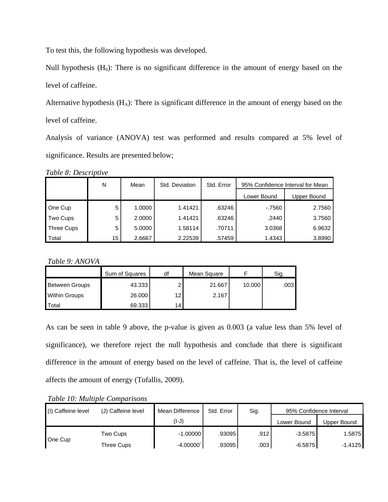
A post-hoc analysis by Bonferroni showed that there was significant difference in the amount of
energy for one cup and three cups; two cups and three cups but no significant difference in the
amount of energy between one cup and two cups.
Question 6:
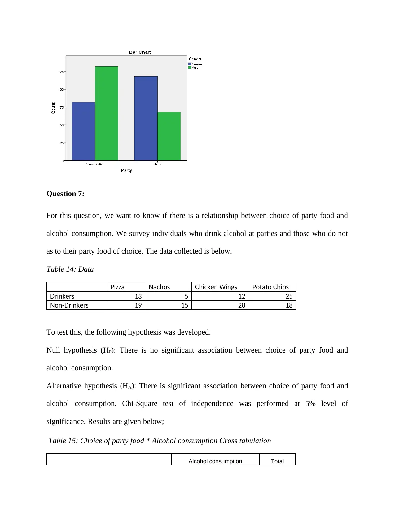
Prior to an election, a survey was conducted to see if choice of political party depends on gender.
The following data was collected from the survey:
Table 11: Data
Liberal Conservative
Female 118 82
Male 68 132
To test this, the following hypothesis was developed.
Three Cups -3.00000* .93095 .022 -5.5875 -.4125
Three Cups One Cup 4.00000* .93095 .003 1.4125 6.5875
Two Cups 3.00000* .93095 .022 .4125 5.5875
*. The mean difference is significant at the 0.05 level.
A post-hoc analysis by Bonferroni showed that there was significant difference in the amount of
energy for one cup and three cups; two cups and three cups but no significant difference in the
amount of energy between one cup and two cups.
Question 6:
Prior to an election, a survey was conducted to see if choice of political party depends on gender.
The following data was collected from the survey:
Table 11: Data
Liberal Conservative
Female 118 82
Male 68 132
To test this, the following hypothesis was developed.
Paraphrase This Document
Need a fresh take? Get an instant paraphrase of this document with our AI Paraphraser
Null hypothesis (H0): There is no significant association between political party one is and the
gender of the person.
Alternative hypothesis (HA): There is significant association between political party one is and
the gender of the person.
Chi-Square test of independence was performed at 5% level of significance. Results are given
below;
Table 12:Party * Gender Cross tabulation
Gender Total
Female Male
Party Conservative 82 132 214
Liberal 118 68 186
Total 200 200 400
Table 13: Chi-Square Tests
Value df Asymp. Sig. (2-
sided)
Exact Sig. (2-
sided)
Exact Sig. (1-
sided)
Pearson Chi-Square 25.123a 1 .000
Continuity Correctionb 24.128 1 .000
Likelihood Ratio 25.399 1 .000
Fisher's Exact Test .000 .000
N of Valid Cases 400
a. 0 cells (0.0%) have expected count less than 5. The minimum expected count is 93.00.
b. Computed only for a 2x2 table
As can be seen in table 13 above, the p-value is given as 0.000 (a value less than 5% level of
significance), we therefore reject the null hypothesis and conclude that there is significant
association between political party one is and the gender of the person. Majority of females
associate with Liberal party while majority of males associate with Conservative party.
Question 7:
For this question, we want to know if there is a relationship between choice of party food and
alcohol consumption. We survey individuals who drink alcohol at parties and those who do not
as to their party food of choice. The data collected is below.
Table 14: Data
Pizza Nachos Chicken Wings Potato Chips
Drinkers 13 5 12 25
Non-Drinkers 19 15 28 18
To test this, the following hypothesis was developed.
Null hypothesis (H0): There is no significant association between choice of party food and
alcohol consumption.
Alternative hypothesis (HA): There is significant association between choice of party food and
alcohol consumption. Chi-Square test of independence was performed at 5% level of
significance. Results are given below;
Table 15: Choice of party food * Alcohol consumption Cross tabulation
Alcohol consumption Total
⊘ This is a preview!⊘
Do you want full access?
Subscribe today to unlock all pages.
Trusted by 1+ million students worldwide
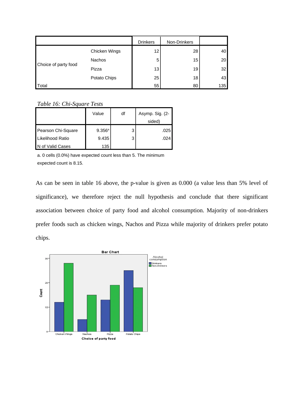
Drinkers Non-Drinkers
Choice of party food
Chicken Wings 12 28 40
Nachos 5 15 20
Pizza 13 19 32
Potato Chips 25 18 43
Total 55 80 135
Table 16: Chi-Square Tests
Value df Asymp. Sig. (2-
sided)
Pearson Chi-Square 9.356a 3 .025
Likelihood Ratio 9.435 3 .024
N of Valid Cases 135
a. 0 cells (0.0%) have expected count less than 5. The minimum
expected count is 8.15.
As can be seen in table 16 above, the p-value is given as 0.000 (a value less than 5% level of
significance), we therefore reject the null hypothesis and conclude that there significant
association between choice of party food and alcohol consumption. Majority of non-drinkers
prefer foods such as chicken wings, Nachos and Pizza while majority of drinkers prefer potato
chips.
Paraphrase This Document
Need a fresh take? Get an instant paraphrase of this document with our AI Paraphraser
Question 8:
For question 8, a faculty member believes that students’ final grades are by both, their IQ, and
the engagement they demonstrate in the class (via Blackboard checking).
Table 17: Data
Final Grade Blackboard checking IQ
91 60 134
70 22 107
84 41 120
56 10 102
49 2 105
78 33 110
94 35 105
68 20 100
This was tested using a regression analysis. The results are presented below;
Table 18: Model Summary
Model R R Square Adjusted R
Square
Std. Error of the
Estimate
1 .972a .944 .922 4.49647
a. Predictors: (Constant), IQ, Blackboard checking
From table 18 above, we can see the value of R-Square to be 0.944; this implies that
94.4% of the variation in the dependent variable (final grades) is explained by the two independe
nt variables (IQ and the engagement they demonstrate in the class) in the model.
Table 19: ANOVAa
Model Sum of Squares df Mean Square F Sig.
1
Regression 1704.409 2 852.205 42.150 .001b
Residual 101.091 5 20.218
Total 1805.500 7
a. Dependent Variable: Final Grade
b. Predictors: (Constant), IQ, Blackboard checking
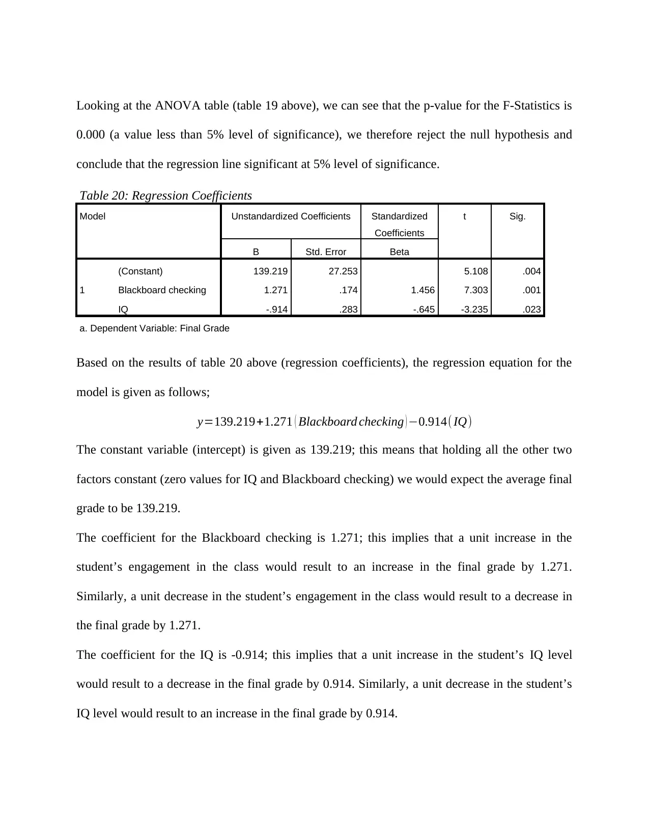
Looking at the ANOVA table (table 19 above), we can see that the p-value for the F-Statistics is
0.000 (a value less than 5% level of significance), we therefore reject the null hypothesis and
conclude that the regression line significant at 5% level of significance.
Table 20: Regression Coefficients
Model Unstandardized Coefficients Standardized
Coefficients
t Sig.
B Std. Error Beta
1
(Constant) 139.219 27.253 5.108 .004
Blackboard checking 1.271 .174 1.456 7.303 .001
IQ -.914 .283 -.645 -3.235 .023
a. Dependent Variable: Final Grade
Based on the results of table 20 above (regression coefficients), the regression equation for the
model is given as follows;
y=139.219+1.271 ( Blackboard checking ) −0.914( IQ)
The constant variable (intercept) is given as 139.219; this means that holding all the other two
factors constant (zero values for IQ and Blackboard checking) we would expect the average final
grade to be 139.219.
The coefficient for the Blackboard checking is 1.271; this implies that a unit increase in the
student’s engagement in the class would result to an increase in the final grade by 1.271.
Similarly, a unit decrease in the student’s engagement in the class would result to a decrease in
the final grade by 1.271.
The coefficient for the IQ is -0.914; this implies that a unit increase in the student’s IQ level
would result to a decrease in the final grade by 0.914. Similarly, a unit decrease in the student’s
IQ level would result to an increase in the final grade by 0.914.
⊘ This is a preview!⊘
Do you want full access?
Subscribe today to unlock all pages.
Trusted by 1+ million students worldwide
1 out of 17
Related Documents


![Statistical Analysis and Hypothesis Testing Assignment - [Course Name]](/_next/image/?url=https%3A%2F%2Fdesklib.com%2Fmedia%2Fimages%2Fgm%2F139f8470657347ce91a85f124f52b5d8.jpg&w=256&q=75)

Your All-in-One AI-Powered Toolkit for Academic Success.
+13062052269
info@desklib.com
Available 24*7 on WhatsApp / Email
![[object Object]](/_next/static/media/star-bottom.7253800d.svg)
Unlock your academic potential
Copyright © 2020–2026 A2Z Services. All Rights Reserved. Developed and managed by ZUCOL.