Psychological Well-being: Psy2530 Descriptive Statistics Problem Set 1

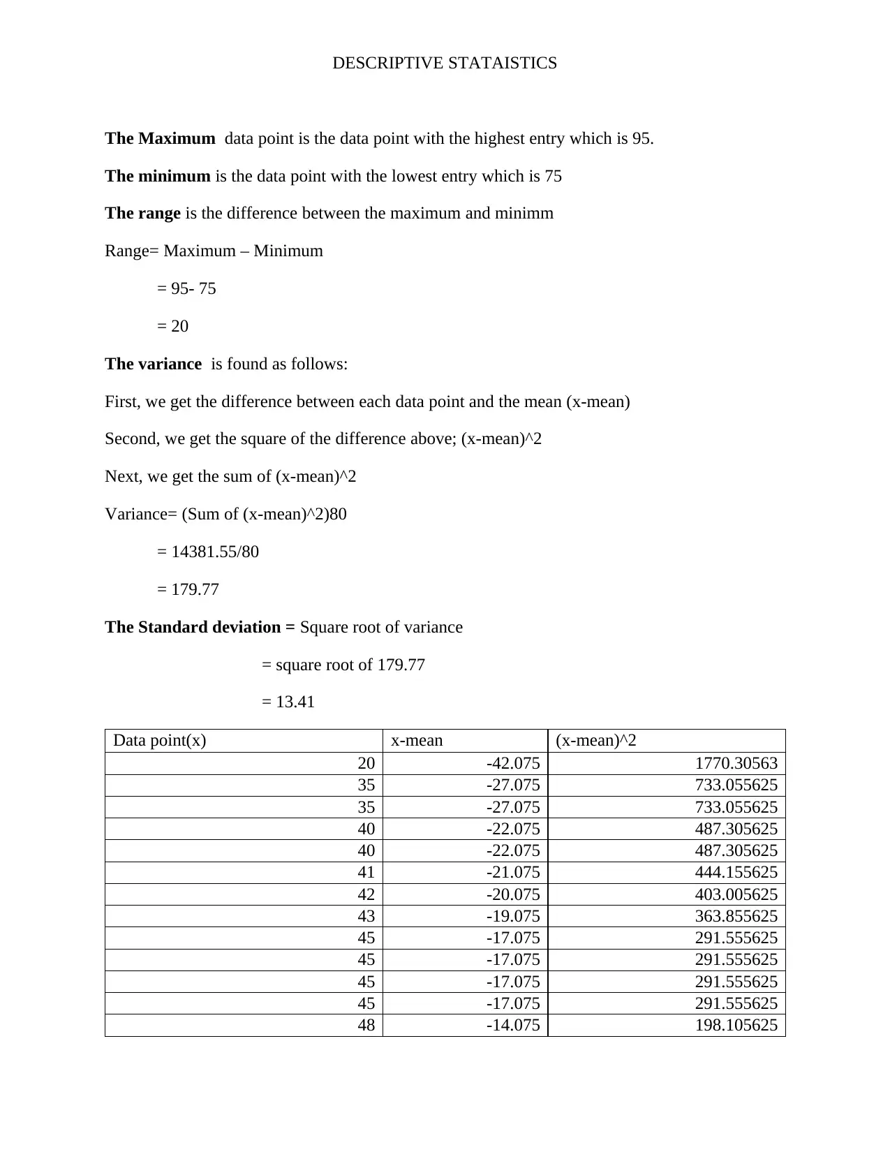
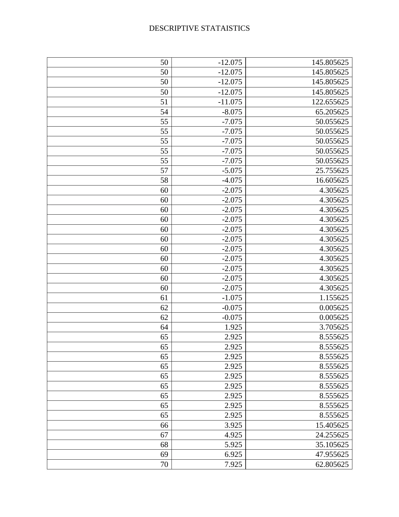
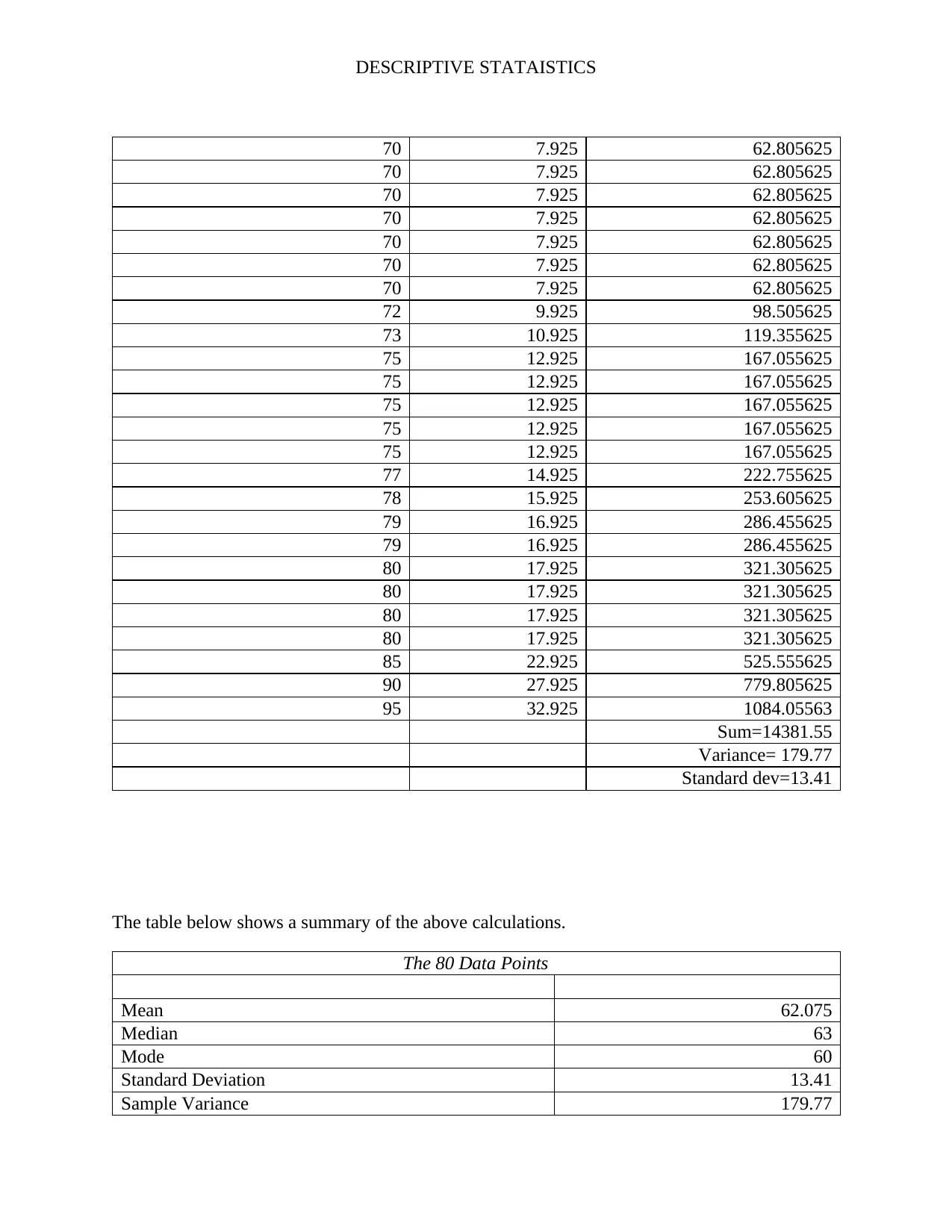
This assignment analyzes a dataset of 80 students' psychological well-being scores to investigate potential gender differences. It begins by classifying the data as a sample or population based on the context. The independent variable (gender) and dependent variable (level of psychological well-being, a continuous variable) are identified. A frequency distribution table is constructed, including absolute, cumulative absolute, and relative frequencies. Histograms are created to visualize the data. Measures of central tendency (mean, median, mode) and variability (range, variance, standard deviation) are calculated. Boxplots and stem-and-leaf displays are generated to represent the data visually, and conclusions are drawn regarding gender differences in well-being and the presence of outliers. The solution includes the R code used for generating the visualizations.

Running Head: DESCRIPTIVE STATAISTICS
1
DESCRIPTIVE STATAISTICS
Name of student:
Name of Institution:
Date:
Author Note:

DESCRIPTIVE STATAISTICS
Psy2530- Problem Set #1
1) The data presented above could be considered a sample or population. Using the
information given in the introductory paragraph, explain to me in what context these 80
data points would represent a population and an example where they would represent a
sample.
Solution: The data represented above can be considered as a population if the study
involves a small group of individuals. For example, the investigation of the existence of
gender difference in the level of psychological well- being among the staff members of a
school. In the scenario of a staff member of a school, if the total number of staff members
in a school is 80, then the data set can be considered as a population. On the other hand, if
the investigation involves gender differences in a school with many students and staff
members, then the data set can be considered as a sample of the whole population in that
school. A sample is a subset of a population (Libman & Zipora, 2010)
2) a) What is the independent variable in this study?
Solution: The independent variable is gender (men or women).
b) What is the dependent variable? Is it a continuous or discrete variable? What is the
scale of measurement for this variable?
Solution: The dependent variable is the level of psychological well- being. The dependent
variable is continuous. The variable is measured on a numerical scale.
3) Construct a frequency distribution table with columns for a) absolute frequencies, b)
cumulative absolute frequencies and c) relative frequencies using all 80 data points.
Create a histogram illustrating the absolute frequencies. Be sure to calculate and
present all measures of central tendency and variability for this distribution, i.e., mean,
median, mode, range, variance, and standard deviation.

DESCRIPTIVE STATAISTICS
Solution: Frequency tables for Women
Frequency table for women shows the number of women for each category of age groups. The
age groups have been divided into classes with a width of 10. The column of “lower limit” below
represents the lower limit of each class that starts from 0, and the “upper limit” shows the upper
limit for each class which starts at 19. The absolute frequency is found by simply counting the
number of individuals whose ages fall in the age bracket (class). Cumulative frequency has been
obtained by adding up the absolute frequencies for each class. Since the total is 80, the
percentage (%) has been obtained by dividing each of the values in the cumulative frequency
column by 80 and multiplying by 100.
Absolute frequency = Count of individuals in each class
Cumulative frequency for class n = Cumulative of class (n-1) + Absolute Frequency of class n.
For example: Cumulative Frequency for class (70-79) = Cumulative Frequency of class (60-69)
+ Absolute Frequency of class (70-79).
That is; 27 + 10= 37
Lower limit Upper Limit Absolute
Frequency
Cumulative
Frequency
Cumulative %
0 19 0 0 0.00%
20 29 0 0 0.00%
30 39 0 0 0.00%
40 49 2 2 5.00%
50 59 7 9 22.50%
60 69 18 27 67.50%
70 79 10 37 92.50%
80 89 2 39 97.50%
90 99 1 40 100.00%
More 0 100.00%
Solution: Frequency tables for Men
Absolute frequency = Count of individuals in each class
Cumulative frequency for class n = Cumulative of class (n-1) + Absolute Frequency of class n.
For example: Cumulative Frequency for class (70-79) = Cumulative Frequency of class (60-69)
+ Absolute Frequency of class (70-79).

DESCRIPTIVE STATAISTICS
That is; 27 + 9 = 36
Lower Limit upper
limit
Absolute
Frequency
Cumulative
Frequency
Cumulative %
0 19 0 0 0.00%
20 29 1 1 2.50%
30 39 2 3 7.50%
40 49 8 11 27.50%
50 59 6 17 42.50%
60 69 10 27 67.50%
70 79 9 36 90.00%
80 89 3 39 97.50%
90 99 1 40 100.00%
More 0 100.00%
Solution: Histograms
The histogram is a pictorial representation of the frequencies of each each clsas. The histogram
represents a representation of class frequency against mid class.
Class width= (Lower Limit + Upper Limit)/2
Class Mid- class Frequency
0-19 9.5 Absolute Frequency
20-29 24.5 0
30-39 34.5 0
40-49 44.5 0
50-59 54.5 2
60-69 64.5 7
70-79 74.5 18
8089 84.5 10
90-99 94.5 2
More 1
0

DESCRIPTIVE STATAISTICS
69 79 59 49 89 99 19 29 39 More
0
2
4
6
8
10
12
14
16
18
20
0.00%
20.00%
40.00%
60.00%
80.00%
100.00%
120.00%
Histogram showing the level Psychological
Well- being of Women
Frequency
Cumulative %
upper limit
Frequency
Class Mid- class Frequency
0-19 9.5 Absolute Frequency
20-29 24.5 0
30-39 34.5 1
40-49 44.5 2
50-59 54.5 8
60-69 64.5 6
70-79 74.5 10
8089 84.5 9
90-99 94.5 3
More 1
0

DESCRIPTIVE STATAISTICS
69 79 49 59 89 39 29 99 19 More
0
2
4
6
8
10
12
0.00%
20.00%
40.00%
60.00%
80.00%
100.00%
120.00%
Histogram showing theblevel Psychological
Well- being of men
Frequency
Cumulative %
upper limit
Frequency
Solution: Measures of central tendency and variability
Mean= (sum of all data points/80)
Mean = (70 + 80 + 77 + 66 + 60 + 70 + 65 + 65 + 60 + 50 + 51 + 80 + 60 + 65 + 65 + 64 + 69 +
54 + 61 + 57 + 73 + 43 + 75 + 60 + 90 + 70 + 65 + 55 + 55 + 62 + 70 + 45 + 75 + 65 + 50 + 70 +
68 + 67 + 60 + 79 + 75 + 50 + 58 + 41 + 60 + 72 + 60 + 70 + 40 + 79 + 80 + 55 + 60 + 70+ 50 +
65 + 42+ 48+ 70+ 60+ 80+ 45+ 60+ 40+ 45+ 55+ 65+ 55+ 65+ 62+ 20+ 75+ 78+ 95+ 45+ 60+
85+ 35+ 35+ 75)/80
= (4966)/80
= 62.075
Median= The middle number. Median is found by arranging the number from the smallest to the
largest and picking middle number. Since the total number of data points is even (80), the
median will fall in the 40th and 41st data points. The data points are arranged as follows:
The 40th data point = 62 and the 41st data point = 64
Therefore; the median = (62+64)/2 = 63

DESCRIPTIVE STATAISTICS
Position Data point

DESCRIPTIVE STATAISTICS
1 20
2 35
3 35
4 40
5 40
6 41
7 42
8 43
9 45
10 45
11 45
12 45
13 48
14 50
15 50
16 50
17 50
18 51
19 54
20 55
21 55
22 55
23 55
24 55
25 57
26 58
27 60
28 60
29 60
30 60
31 60
32 60
33 60
34 60
35 60
36 60
37 60
38 61
39 62
40 62
41 64
42 65

DESCRIPTIVE STATAISTICS
43 65
44 65
45 65
46 65
47 65
48 65
49 65
50 65
51 66
52 67
53 68
54 69
55 70
56 70
57 70
58 70
59 70
60 70
61 70
62 70
63 72
64 73
65 75
66 75
67 75
68 75
69 75
70 77
71 78
72 79
73 79
74 80
75 80
76 80
77 80
78 85
79 90
80 95
The mode is the data point with the highest number of appearances. From the data points, it is
clear that the data point with the highest number of appearance is 60.

DESCRIPTIVE STATAISTICS
The Maximum data point is the data point with the highest entry which is 95.
The minimum is the data point with the lowest entry which is 75
The range is the difference between the maximum and minimm
Range= Maximum – Minimum
= 95- 75
= 20
The variance is found as follows:
First, we get the difference between each data point and the mean (x-mean)
Second, we get the square of the difference above; (x-mean)^2
Next, we get the sum of (x-mean)^2
Variance= (Sum of (x-mean)^2)80
= 14381.55/80
= 179.77
The Standard deviation = Square root of variance
= square root of 179.77
= 13.41
Data point(x) x-mean (x-mean)^2
20 -42.075 1770.30563
35 -27.075 733.055625
35 -27.075 733.055625
40 -22.075 487.305625
40 -22.075 487.305625
41 -21.075 444.155625
42 -20.075 403.005625
43 -19.075 363.855625
45 -17.075 291.555625
45 -17.075 291.555625
45 -17.075 291.555625
45 -17.075 291.555625
48 -14.075 198.105625

DESCRIPTIVE STATAISTICS
50 -12.075 145.805625
50 -12.075 145.805625
50 -12.075 145.805625
50 -12.075 145.805625
51 -11.075 122.655625
54 -8.075 65.205625
55 -7.075 50.055625
55 -7.075 50.055625
55 -7.075 50.055625
55 -7.075 50.055625
55 -7.075 50.055625
57 -5.075 25.755625
58 -4.075 16.605625
60 -2.075 4.305625
60 -2.075 4.305625
60 -2.075 4.305625
60 -2.075 4.305625
60 -2.075 4.305625
60 -2.075 4.305625
60 -2.075 4.305625
60 -2.075 4.305625
60 -2.075 4.305625
60 -2.075 4.305625
60 -2.075 4.305625
61 -1.075 1.155625
62 -0.075 0.005625
62 -0.075 0.005625
64 1.925 3.705625
65 2.925 8.555625
65 2.925 8.555625
65 2.925 8.555625
65 2.925 8.555625
65 2.925 8.555625
65 2.925 8.555625
65 2.925 8.555625
65 2.925 8.555625
65 2.925 8.555625
66 3.925 15.405625
67 4.925 24.255625
68 5.925 35.105625
69 6.925 47.955625
70 7.925 62.805625

DESCRIPTIVE STATAISTICS
70 7.925 62.805625
70 7.925 62.805625
70 7.925 62.805625
70 7.925 62.805625
70 7.925 62.805625
70 7.925 62.805625
70 7.925 62.805625
72 9.925 98.505625
73 10.925 119.355625
75 12.925 167.055625
75 12.925 167.055625
75 12.925 167.055625
75 12.925 167.055625
75 12.925 167.055625
77 14.925 222.755625
78 15.925 253.605625
79 16.925 286.455625
79 16.925 286.455625
80 17.925 321.305625
80 17.925 321.305625
80 17.925 321.305625
80 17.925 321.305625
85 22.925 525.555625
90 27.925 779.805625
95 32.925 1084.05563
Sum=14381.55
Variance= 179.77
Standard dev=13.41
The table below shows a summary of the above calculations.
The 80 Data Points
Mean 62.075
Median 63
Mode 60
Standard Deviation 13.41
Sample Variance 179.77