University Psychology Practical: Correlation and Regression Analysis

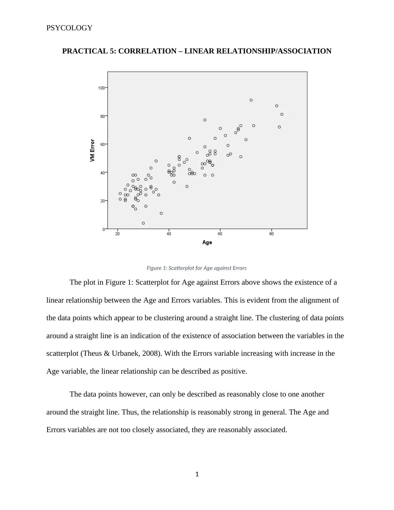
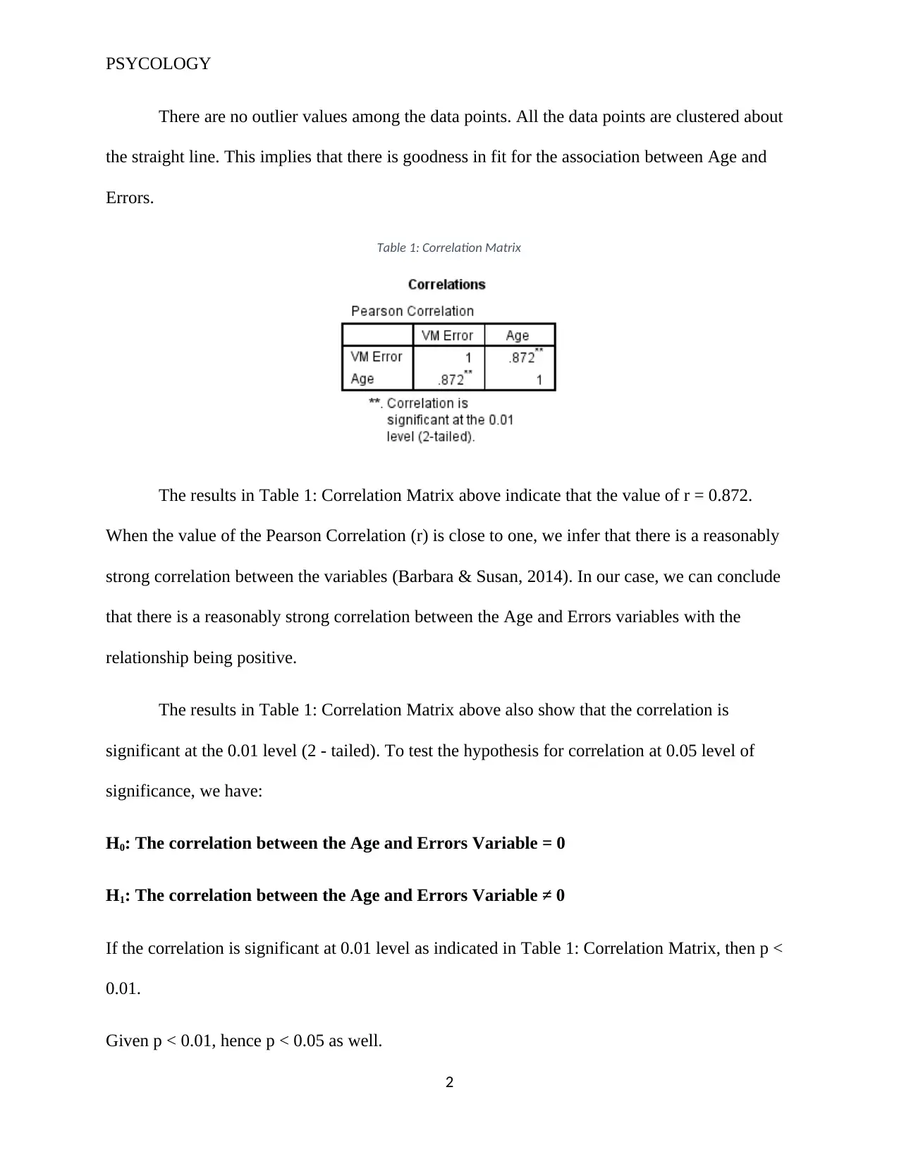
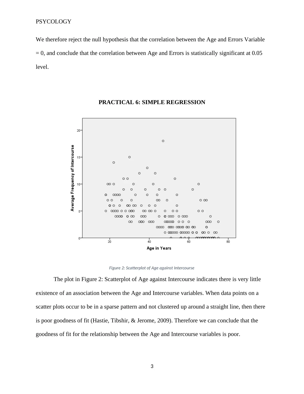
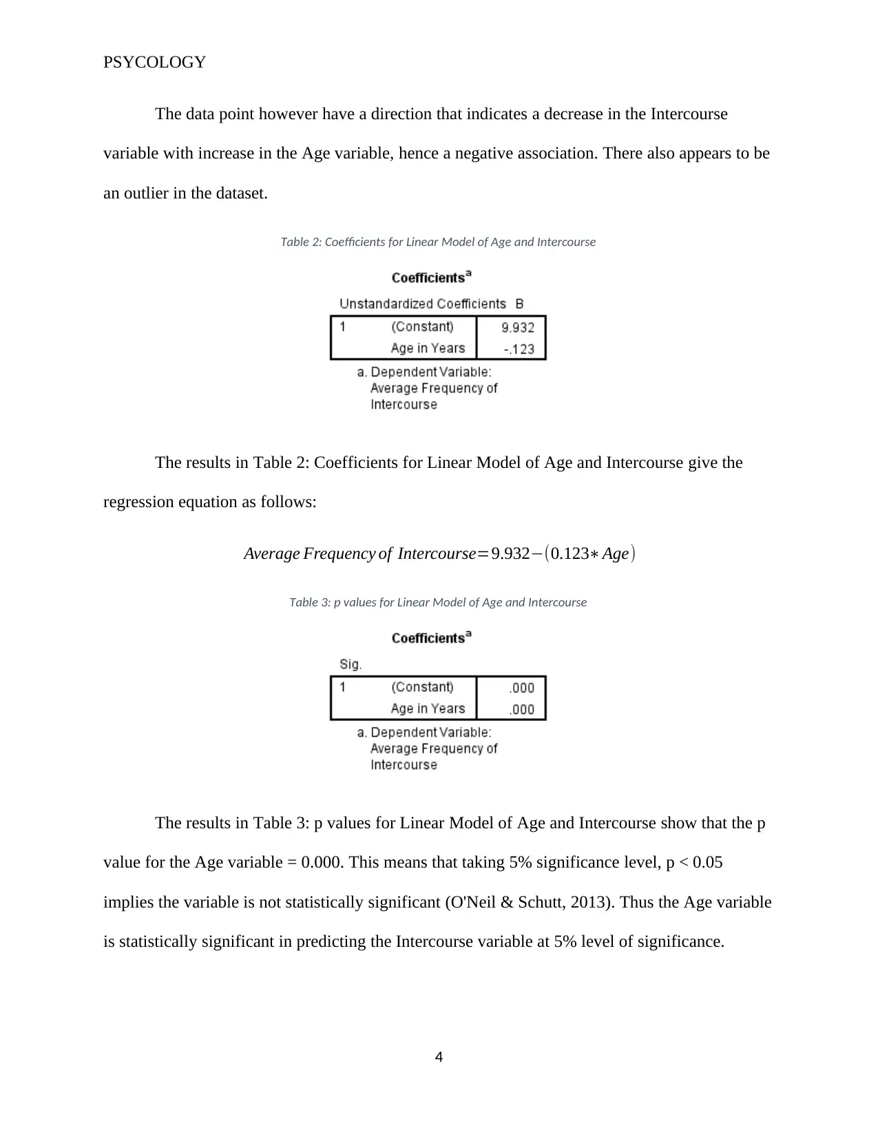
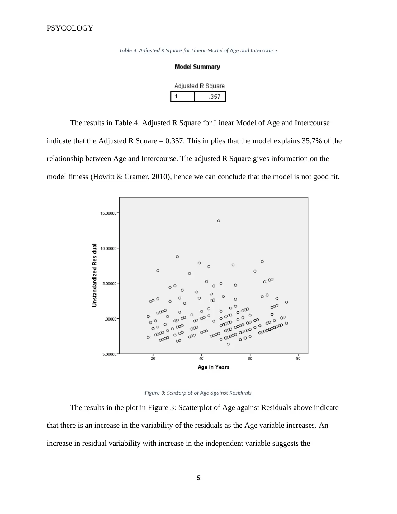
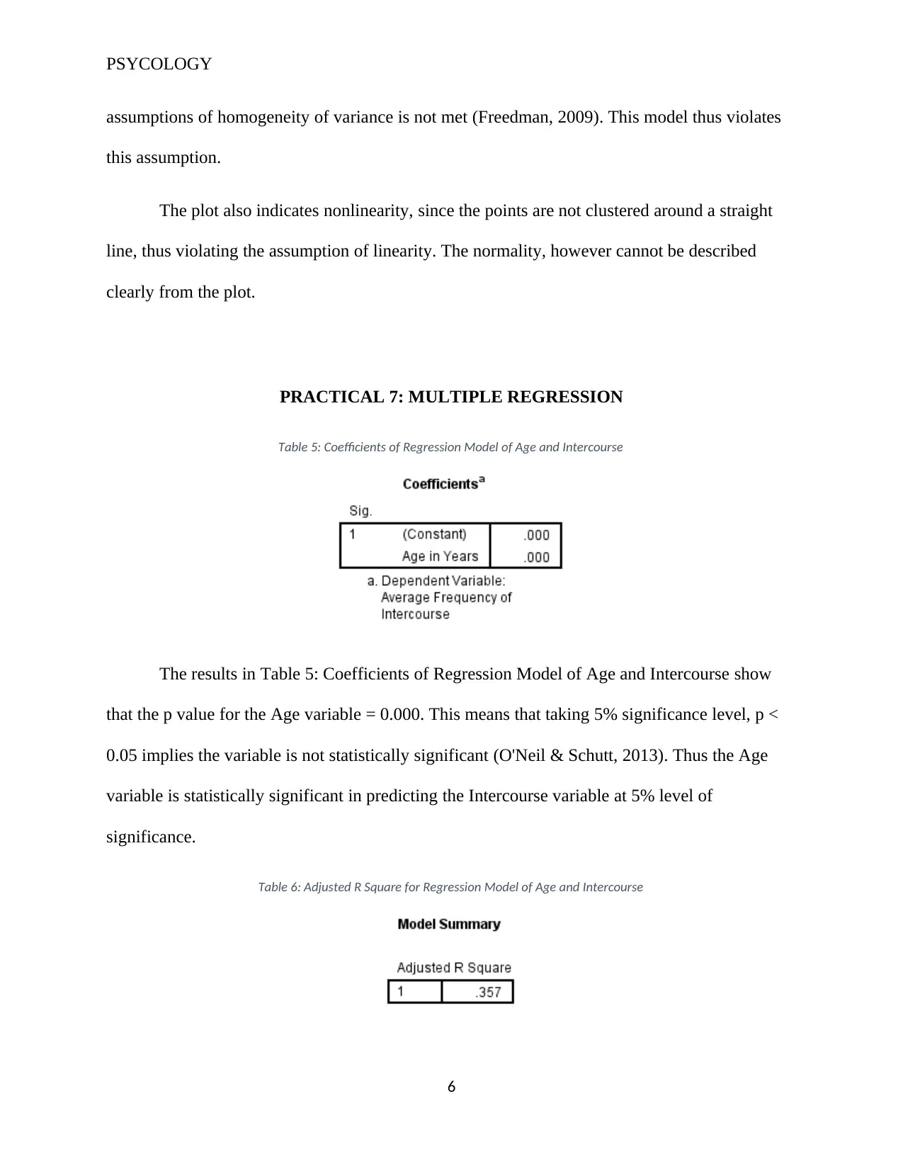
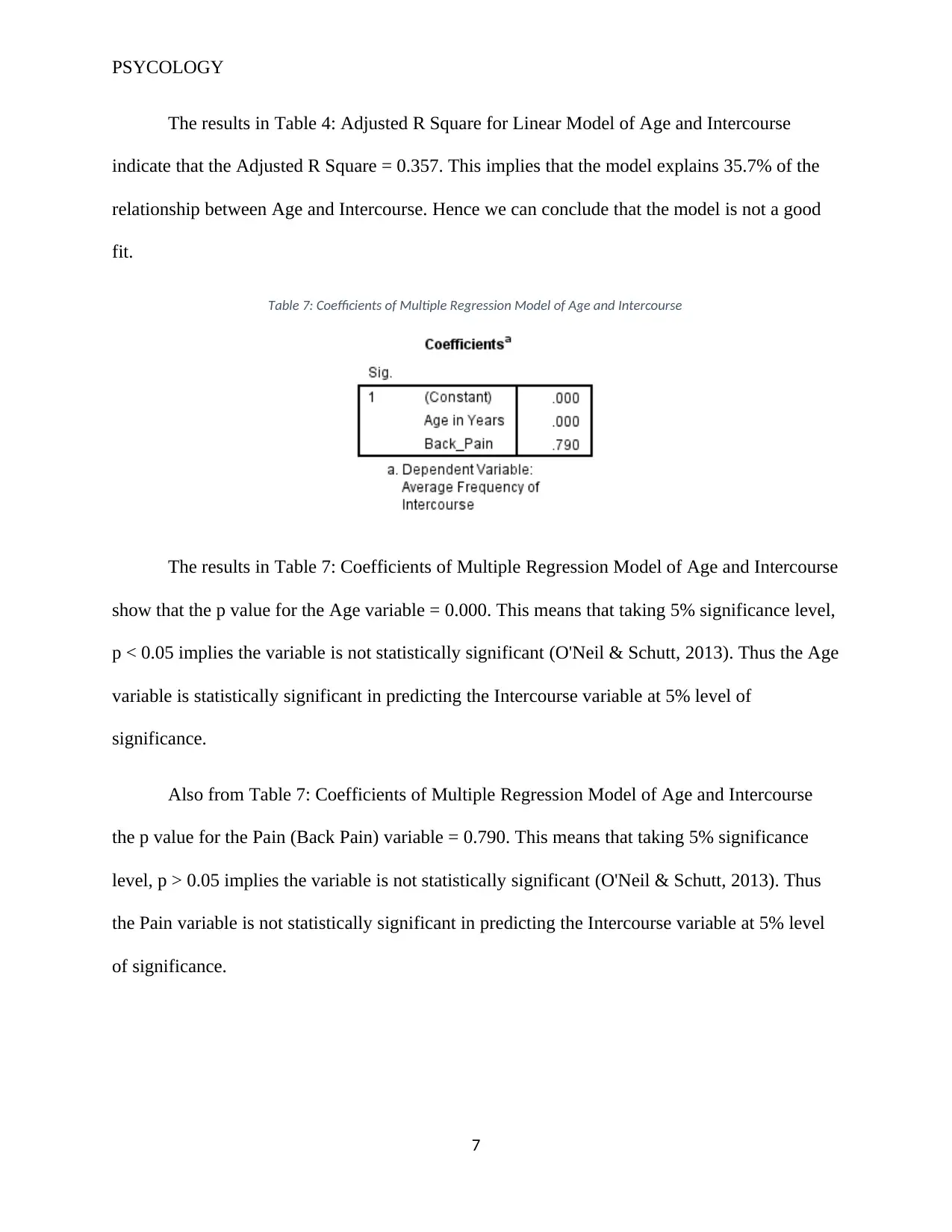
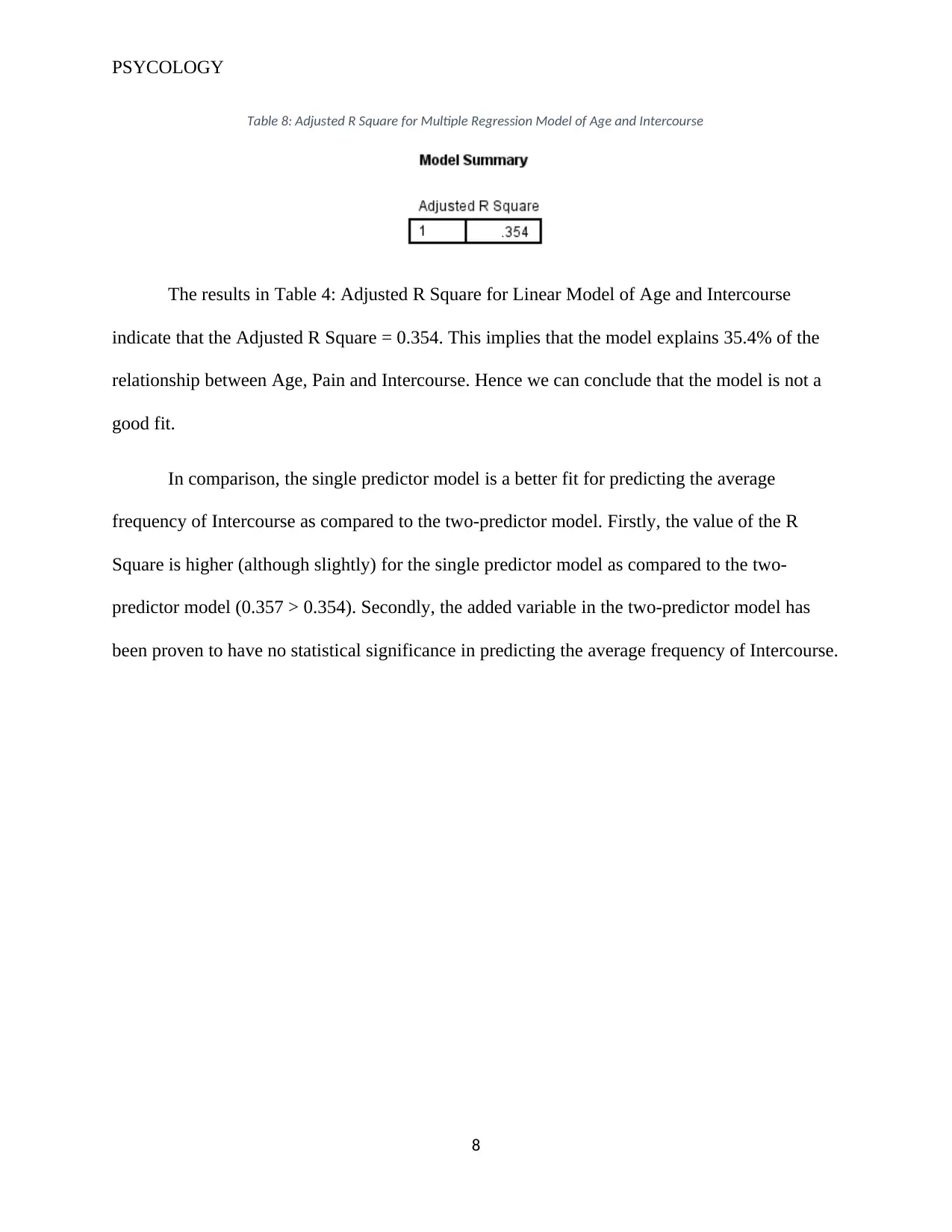
This psychology practical assignment explores correlation and regression analysis using real-world data. The assignment analyzes scatterplots to identify linear relationships between variables such as age and errors, and age and intercourse. It utilizes Pearson correlation to measure the strength and direction of linear relationships, determining statistical significance through hypothesis testing. The assignment also delves into simple and multiple regression models, examining coefficients, p-values, and adjusted R-squared to assess model fit and the predictive power of variables. The analysis includes interpretations of model assumptions, such as homogeneity of variance and linearity, providing a comprehensive understanding of statistical techniques used in psychological research. The document concludes with a comparison of different models and their effectiveness in predicting outcomes.

PSYCOLOGY
PRACTICAL 5: CORRELATION – LINEAR RELATIONSHIP/ASSOCIATION
Figure 1: Scatterplot for Age against Errors
The plot in Figure 1: Scatterplot for Age against Errors above shows the existence of a
linear relationship between the Age and Errors variables. This is evident from the alignment of
the data points which appear to be clustering around a straight line. The clustering of data points
around a straight line is an indication of the existence of association between the variables in the
scatterplot (Theus & Urbanek, 2008). With the Errors variable increasing with increase in the
Age variable, the linear relationship can be described as positive.
The data points however, can only be described as reasonably close to one another
around the straight line. Thus, the relationship is reasonably strong in general. The Age and
Errors variables are not too closely associated, they are reasonably associated.
1

PSYCOLOGY
There are no outlier values among the data points. All the data points are clustered about
the straight line. This implies that there is goodness in fit for the association between Age and
Errors.
Table 1: Correlation Matrix
The results in Table 1: Correlation Matrix above indicate that the value of r = 0.872.
When the value of the Pearson Correlation (r) is close to one, we infer that there is a reasonably
strong correlation between the variables (Barbara & Susan, 2014). In our case, we can conclude
that there is a reasonably strong correlation between the Age and Errors variables with the
relationship being positive.
The results in Table 1: Correlation Matrix above also show that the correlation is
significant at the 0.01 level (2 - tailed). To test the hypothesis for correlation at 0.05 level of
significance, we have:
H0: The correlation between the Age and Errors Variable = 0
H1: The correlation between the Age and Errors Variable ≠ 0
If the correlation is significant at 0.01 level as indicated in Table 1: Correlation Matrix, then p <
0.01.
Given p < 0.01, hence p < 0.05 as well.
2

PSYCOLOGY
We therefore reject the null hypothesis that the correlation between the Age and Errors Variable
= 0, and conclude that the correlation between Age and Errors is statistically significant at 0.05
level.
PRACTICAL 6: SIMPLE REGRESSION
Figure 2: Scatterplot of Age against Intercourse
The plot in Figure 2: Scatterplot of Age against Intercourse indicates there is very little
existence of an association between the Age and Intercourse variables. When data points on a
scatter plots occur to be in a sparse pattern and not clustered up around a straight line, then there
is poor goodness of fit (Hastie, Tibshir, & Jerome, 2009). Therefore we can conclude that the
goodness of fit for the relationship between the Age and Intercourse variables is poor.
3

PSYCOLOGY
The data point however have a direction that indicates a decrease in the Intercourse
variable with increase in the Age variable, hence a negative association. There also appears to be
an outlier in the dataset.
Table 2: Coefficients for Linear Model of Age and Intercourse
The results in Table 2: Coefficients for Linear Model of Age and Intercourse give the
regression equation as follows:
Average Frequency of Intercourse=9.932−(0.123∗Age)
Table 3: p values for Linear Model of Age and Intercourse
The results in Table 3: p values for Linear Model of Age and Intercourse show that the p
value for the Age variable = 0.000. This means that taking 5% significance level, p < 0.05
implies the variable is not statistically significant (O'Neil & Schutt, 2013). Thus the Age variable
is statistically significant in predicting the Intercourse variable at 5% level of significance.
4

PSYCOLOGY
Table 4: Adjusted R Square for Linear Model of Age and Intercourse
The results in Table 4: Adjusted R Square for Linear Model of Age and Intercourse
indicate that the Adjusted R Square = 0.357. This implies that the model explains 35.7% of the
relationship between Age and Intercourse. The adjusted R Square gives information on the
model fitness (Howitt & Cramer, 2010), hence we can conclude that the model is not good fit.
Figure 3: Scatterplot of Age against Residuals
The results in the plot in Figure 3: Scatterplot of Age against Residuals above indicate
that there is an increase in the variability of the residuals as the Age variable increases. An
increase in residual variability with increase in the independent variable suggests the
5

PSYCOLOGY
assumptions of homogeneity of variance is not met (Freedman, 2009). This model thus violates
this assumption.
The plot also indicates nonlinearity, since the points are not clustered around a straight
line, thus violating the assumption of linearity. The normality, however cannot be described
clearly from the plot.
PRACTICAL 7: MULTIPLE REGRESSION
Table 5: Coefficients of Regression Model of Age and Intercourse
The results in Table 5: Coefficients of Regression Model of Age and Intercourse show
that the p value for the Age variable = 0.000. This means that taking 5% significance level, p <
0.05 implies the variable is not statistically significant (O'Neil & Schutt, 2013). Thus the Age
variable is statistically significant in predicting the Intercourse variable at 5% level of
significance.
Table 6: Adjusted R Square for Regression Model of Age and Intercourse
6

PSYCOLOGY
The results in Table 4: Adjusted R Square for Linear Model of Age and Intercourse
indicate that the Adjusted R Square = 0.357. This implies that the model explains 35.7% of the
relationship between Age and Intercourse. Hence we can conclude that the model is not a good
fit.
Table 7: Coefficients of Multiple Regression Model of Age and Intercourse
The results in Table 7: Coefficients of Multiple Regression Model of Age and Intercourse
show that the p value for the Age variable = 0.000. This means that taking 5% significance level,
p < 0.05 implies the variable is not statistically significant (O'Neil & Schutt, 2013). Thus the Age
variable is statistically significant in predicting the Intercourse variable at 5% level of
significance.
Also from Table 7: Coefficients of Multiple Regression Model of Age and Intercourse
the p value for the Pain (Back Pain) variable = 0.790. This means that taking 5% significance
level, p > 0.05 implies the variable is not statistically significant (O'Neil & Schutt, 2013). Thus
the Pain variable is not statistically significant in predicting the Intercourse variable at 5% level
of significance.
7

PSYCOLOGY
Table 8: Adjusted R Square for Multiple Regression Model of Age and Intercourse
The results in Table 4: Adjusted R Square for Linear Model of Age and Intercourse
indicate that the Adjusted R Square = 0.354. This implies that the model explains 35.4% of the
relationship between Age, Pain and Intercourse. Hence we can conclude that the model is not a
good fit.
In comparison, the single predictor model is a better fit for predicting the average
frequency of Intercourse as compared to the two-predictor model. Firstly, the value of the R
Square is higher (although slightly) for the single predictor model as compared to the two-
predictor model (0.357 > 0.354). Secondly, the added variable in the two-predictor model has
been proven to have no statistical significance in predicting the average frequency of Intercourse.
8

PSYCOLOGY
References
Barbara, I., & Susan, D. (2014). Introductory Statistics (1st ed.). New York: OpenStax CNX.
Freedman, D. A. (2009). Statistical Models: Theory and Practice. London: Cambridge
University Press.
Hastie, T., Tibshir, R., & Jerome, H. (2009). The Elements of Statistical Learning (2nd ed.). New
York: Springer.
Howitt, D., & Cramer, D. (2010). Introduction to Descriptive Statistics in Psycology, 5th
Edition. New York: Prentice Hall.
O'Neil, C., & Schutt, R. (2013). Doing Data Science (3rd ed.). London: O'Reily.
Theus, M., & Urbanek, S. (2008). Inteactive Graphics For Data Analysis (1st ed.). Boca Raton:
CRC Press.
9

PSYCOLOGY
10