Psychology Portfolio: Exercises on Ethics, Statistics, and Research
VerifiedAdded on 2023/01/09
|33
|7066
|93
Portfolio
AI Summary
This psychology portfolio comprises several exercises covering key aspects of psychological research. Exercise 1 focuses on the BPS code of ethics, exploring ethical principles like independence, competence, and transparency, and analyzing studies that adhere to or deviate from these guidelines. Exercise 2 delves into statistical analysis, specifically factorial ANOVA, to investigate the impact of reward and task emotion on procrastination, including descriptive statistics and multiple comparisons. Exercise 3 presents ANCOVA and one-way ANOVA analyses to examine the effect of video game training on divided attention, incorporating descriptive statistics and between-subjects effects. Finally, Exercise 4 provides an overview of research methodology. The portfolio includes detailed analyses, tables, and recommendations, offering a comprehensive understanding of research design, ethical considerations, and statistical techniques commonly used in psychology.

PORTFOLIO
Paraphrase This Document
Need a fresh take? Get an instant paraphrase of this document with our AI Paraphraser
Table of Contents
EXERCISE 1...................................................................................................................................2
Reflection.........................................................................................................................................2
EXERCISE 2...................................................................................................................................4
Descriptive statistics........................................................................................................................4
Factorial ANOVA............................................................................................................................5
Recommendation.............................................................................................................................7
EXERCISE 3...................................................................................................................................9
A. ANCOVA Analysis................................................................................................................9
B. One-way ANOVA Analysis..................................................................................................12
MANOVA exercise.......................................................................................................................13
C. Descriptive statistics.............................................................................................................13
D. MANOVA Analysis.............................................................................................................14
E. Explanation............................................................................................................................15
EXERCISE-4.................................................................................................................................16
Introduction....................................................................................................................................16
METHOD......................................................................................................................................17
RESULTS......................................................................................................................................17
DISCUSSION................................................................................................................................19
REFERENCES..............................................................................................................................20
APPENDIX....................................................................................................................................21
APPENDIX-1............................................................................................................................21
APPENDIX-2............................................................................................................................24
APPENDIX-3............................................................................................................................27
1
EXERCISE 1
Reflection
BPS code of ethics is a full fledged designed code of ethics which guide all the members of
British Psychological Society to carry out their professional conduct. These codes help
psychologists to ensure the ethical treatment of participants. In this reflection multiple studies
which are previously published will be used to show that how data from participants is gathered
without crossing boundaries of ethics.
There are major principles which help in best practice in ethics review; these four principles
include independence, competence, facilitation and transparency & accountability. The first
principle of independence states that the virtue of review of ethics must be independent from the
research itself so that any conflict of interest between researchers and the auditor who is
reviewing the ethics protocol must work between governed structures. This principle further adds
that the person who is investigating the ethics review protocol must be different and independent
from the investigator as by this way ethical conduct of a study can be ensured.
Another principle of BPS code of ethics is competence which states the ethics review
protocol of a research must be investigated by a competent body. The investigators who can form
this body of evaluating ethics review protocol must have proper expertise and must have a proper
training in this process. This principle has the agenda that every research must be checked by
competent reviewers so that ethical treatment of participants can be ensured.
Third principle of BPS codes of ethics is Facilitation; under this principle the review body of
ethics must facilitate the researcher to educate them about the ethical implications which their
research requires it imply. The vision of this principle is to invoke the responsibility of ethics
review body to educate and support the researchers.
The fourth and last principle of BPS code of ethics is transparency and accountability. This
principle states that the process of reviewing the ethical protocol of a study must be accountable
and open for scrutiny so that whenever any misleading ethics review can be undertaken it can be
appropriately located by the scrutiny process. This principle ensures transparent ethics review.
All the above principles of BPS code ensure informed consent, confidentiality, deception,
debriefing and right to withdraw elements in a research.
2
⊘ This is a preview!⊘
Do you want full access?
Subscribe today to unlock all pages.
Trusted by 1+ million students worldwide
It is important for investigators to follow all the BPS codes and principles to ethical conduct
their study. The study conducted by (Best, 2010) and (Repovš and Baddeley, 2006) are good
examples of studies which are undertaken by ensuring every principle of BPS codes. These
studies have asked for a consent from their participants and even have maintained anonymity
while presenting their results of the study. Few more examples of ethical investigations are
(Hafer and Begue, 2005) and (Koole, Greenberg and Pyszczynski, 2006); these studies have also
followed all ethical guidelines.
Out of the published studies stated above, there are few which also has some ethical
pitfalls. The study of (Hafer and Begue, 2005) has avoided the ethical pitfall of reward system
due to which the responses of participants could have become biased. These researchers should
have awareness of complexity of ethics which could have helped them in making better
judgements.
3
Paraphrase This Document
Need a fresh take? Get an instant paraphrase of this document with our AI Paraphraser
EXERCISE 2
A study has been conducted to investigate the effect of reward on procrastination. The
participants of this study will be 60 undergraduate psychology students. These 60 students are
divided into two criterions or factors. The first criteria or variable is the level of reward; there are
three levels or values of this variable which are “no reward”, “small reward” and “large reward”.
The second factor or variable is the task emotion which has two level and those are “pleasant”
and “unpleasant”. All these variables are recorded under a SPSS datasheet which is intended to
be used to conduct Factor ANOVA. This technique of data analysis will help in determining the
impact of reward and emotional manipulation on the procrastination.
The 60 participants are provided with numerical math quizzes and then the data is recorded
based on the time in which each participant has completed their quiz. All the data will be used to
conduct factor ANOVA and to conclude the results.
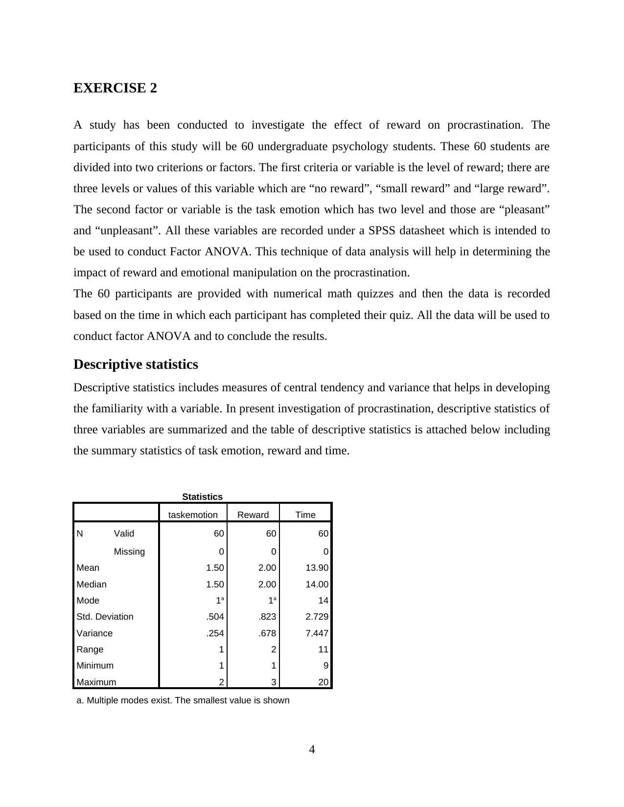
Descriptive statistics
Descriptive statistics includes measures of central tendency and variance that helps in developing
the familiarity with a variable. In present investigation of procrastination, descriptive statistics of
three variables are summarized and the table of descriptive statistics is attached below including
the summary statistics of task emotion, reward and time.
Statistics
taskemotion Reward Time
N Valid 60 60 60
Missing 0 0 0
Mean 1.50 2.00 13.90
Median 1.50 2.00 14.00
Mode 1a 1a 14
Std. Deviation .504 .823 2.729
Variance .254 .678 7.447
Range 1 2 11
Minimum 1 1 9
Maximum 2 3 20
a. Multiple modes exist. The smallest value is shown
4
A study has been conducted to investigate the effect of reward on procrastination. The
participants of this study will be 60 undergraduate psychology students. These 60 students are
divided into two criterions or factors. The first criteria or variable is the level of reward; there are
three levels or values of this variable which are “no reward”, “small reward” and “large reward”.
The second factor or variable is the task emotion which has two level and those are “pleasant”
and “unpleasant”. All these variables are recorded under a SPSS datasheet which is intended to
be used to conduct Factor ANOVA. This technique of data analysis will help in determining the
impact of reward and emotional manipulation on the procrastination.
The 60 participants are provided with numerical math quizzes and then the data is recorded
based on the time in which each participant has completed their quiz. All the data will be used to
conduct factor ANOVA and to conclude the results.
Descriptive statistics
Descriptive statistics includes measures of central tendency and variance that helps in developing
the familiarity with a variable. In present investigation of procrastination, descriptive statistics of
three variables are summarized and the table of descriptive statistics is attached below including
the summary statistics of task emotion, reward and time.
Statistics
taskemotion Reward Time
N Valid 60 60 60
Missing 0 0 0
Mean 1.50 2.00 13.90
Median 1.50 2.00 14.00
Mode 1a 1a 14
Std. Deviation .504 .823 2.729
Variance .254 .678 7.447
Range 1 2 11
Minimum 1 1 9
Maximum 2 3 20
a. Multiple modes exist. The smallest value is shown
4
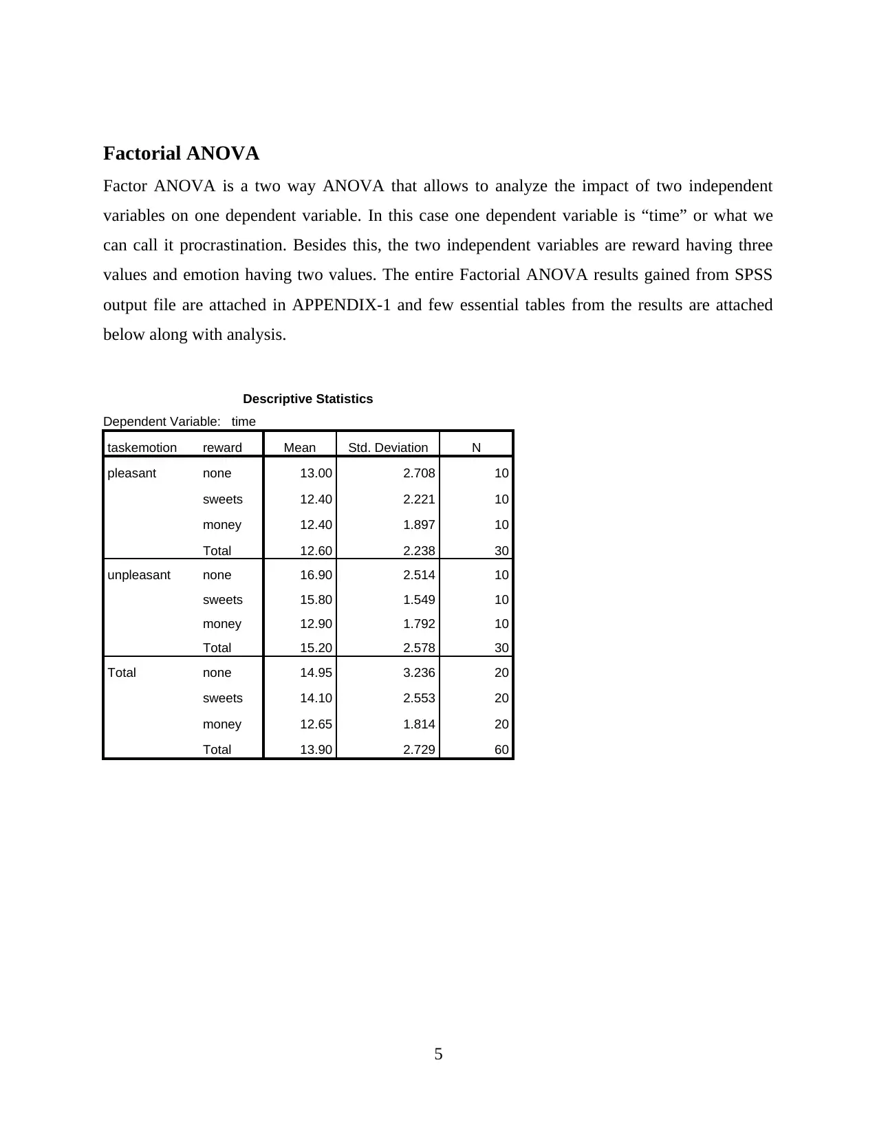
Factorial ANOVA
Factor ANOVA is a two way ANOVA that allows to analyze the impact of two independent
variables on one dependent variable. In this case one dependent variable is “time” or what we
can call it procrastination. Besides this, the two independent variables are reward having three
values and emotion having two values. The entire Factorial ANOVA results gained from SPSS
output file are attached in APPENDIX-1 and few essential tables from the results are attached
below along with analysis.
Descriptive Statistics
Dependent Variable: time
taskemotion reward Mean Std. Deviation N
pleasant none 13.00 2.708 10
sweets 12.40 2.221 10
money 12.40 1.897 10
Total 12.60 2.238 30
unpleasant none 16.90 2.514 10
sweets 15.80 1.549 10
money 12.90 1.792 10
Total 15.20 2.578 30
Total none 14.95 3.236 20
sweets 14.10 2.553 20
money 12.65 1.814 20
Total 13.90 2.729 60
5
⊘ This is a preview!⊘
Do you want full access?
Subscribe today to unlock all pages.
Trusted by 1+ million students worldwide
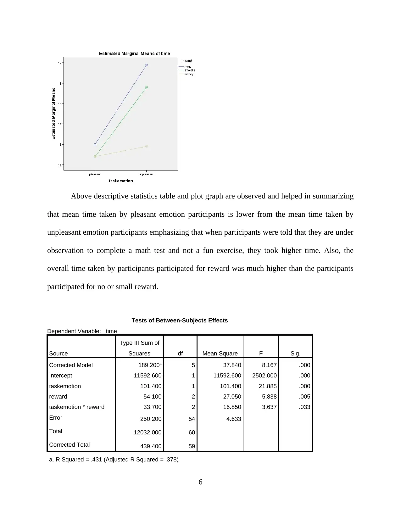
Above descriptive statistics table and plot graph are observed and helped in summarizing
that mean time taken by pleasant emotion participants is lower from the mean time taken by
unpleasant emotion participants emphasizing that when participants were told that they are under
observation to complete a math test and not a fun exercise, they took higher time. Also, the
overall time taken by participants participated for reward was much higher than the participants
participated for no or small reward.
Tests of Between-Subjects Effects
Dependent Variable: time
Source
Type III Sum of
Squares df Mean Square F Sig.
Corrected Model 189.200a 5 37.840 8.167 .000
Intercept 11592.600 1 11592.600 2502.000 .000
taskemotion 101.400 1 101.400 21.885 .000
reward 54.100 2 27.050 5.838 .005
taskemotion * reward 33.700 2 16.850 3.637 .033
Error 250.200 54 4.633
Total 12032.000 60
Corrected Total 439.400 59
a. R Squared = .431 (Adjusted R Squared = .378)
6
Paraphrase This Document
Need a fresh take? Get an instant paraphrase of this document with our AI Paraphraser
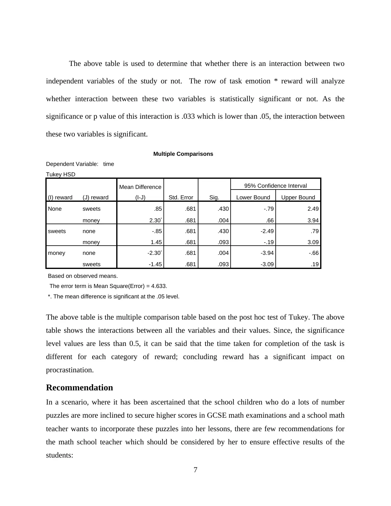
The above table is used to determine that whether there is an interaction between two
independent variables of the study or not. The row of task emotion * reward will analyze
whether interaction between these two variables is statistically significant or not. As the
significance or p value of this interaction is .033 which is lower than .05, the interaction between
these two variables is significant.
Multiple Comparisons
Dependent Variable: time
Tukey HSD
(I) reward (J) reward
Mean Difference
(I-J) Std. Error Sig.
95% Confidence Interval
Lower Bound Upper Bound
None sweets .85 .681 .430 -.79 2.49
money 2.30* .681 .004 .66 3.94
sweets none -.85 .681 .430 -2.49 .79
money 1.45 .681 .093 -.19 3.09
money none -2.30* .681 .004 -3.94 -.66
sweets -1.45 .681 .093 -3.09 .19
Based on observed means.
The error term is Mean Square(Error) = 4.633.
*. The mean difference is significant at the .05 level.
The above table is the multiple comparison table based on the post hoc test of Tukey. The above
table shows the interactions between all the variables and their values. Since, the significance
level values are less than 0.5, it can be said that the time taken for completion of the task is
different for each category of reward; concluding reward has a significant impact on
procrastination.
Recommendation
In a scenario, where it has been ascertained that the school children who do a lots of number
puzzles are more inclined to secure higher scores in GCSE math examinations and a school math
teacher wants to incorporate these puzzles into her lessons, there are few recommendations for
the math school teacher which should be considered by her to ensure effective results of the
students:
7
The math teacher should make sure that her students take this math numeric puzzles as a fun
exercise and not an exercise of testing their math ability. This recommendation is provided after
analyzing the findings which state that students who take their numeric puzzle as a fun exercise
(pleasant) takes lesser mean time to complete the puzzles than the students who consider these
numeric puzzles as a test of their math ability (unpleasant).
Another recommendation for the math teacher is to include some sort of reward against the
completion of math puzzle faster as it will induce the motivation of students and they will
complete the math puzzle in less time. This recommendation is based on the experiment
conducted in the study. The findings of this experiment study stated that the students who were
promised to gain a reward observed to complete the math puzzle a lot faster than the students
who were not participating for any reward.
8
⊘ This is a preview!⊘
Do you want full access?
Subscribe today to unlock all pages.
Trusted by 1+ million students worldwide
EXERCISE 3
A. ANCOVA Analysis
ANCOVA analysis is the one-way ANCOVA analysis in which there are two or more
independent variables with one dependent variable and a covariate. In the present case, the aim
of undertaking an ANCOVA exercise is to investigate whether training in videogames can
improve the people’s ability to divide attention across multiple sources of information. For this,
there are three variables in this study. The first variable is the videogame group, these variable
has three values, first group is the control group who was not given video game training at all,
the second group was the group of people who was given video game training of 10 hours per
week for 3 weeks and the last group is of people who were given training of 20 hours per week
for 3 weeks. Second variable in this study is the divided attention score which is a scale variable
and lastly third variable is age of each participant which is also a scale variable.
For conducting ANCOVA, videogame group is an independent or fixed variable, divided
attention is a dependent variable and age is a covariate. It is assumed for this analysis that the
data set is normal and no normality test is required to be conducted. The results of the analysis
are attached below with analysis.
9
Paraphrase This Document
Need a fresh take? Get an instant paraphrase of this document with our AI Paraphraser
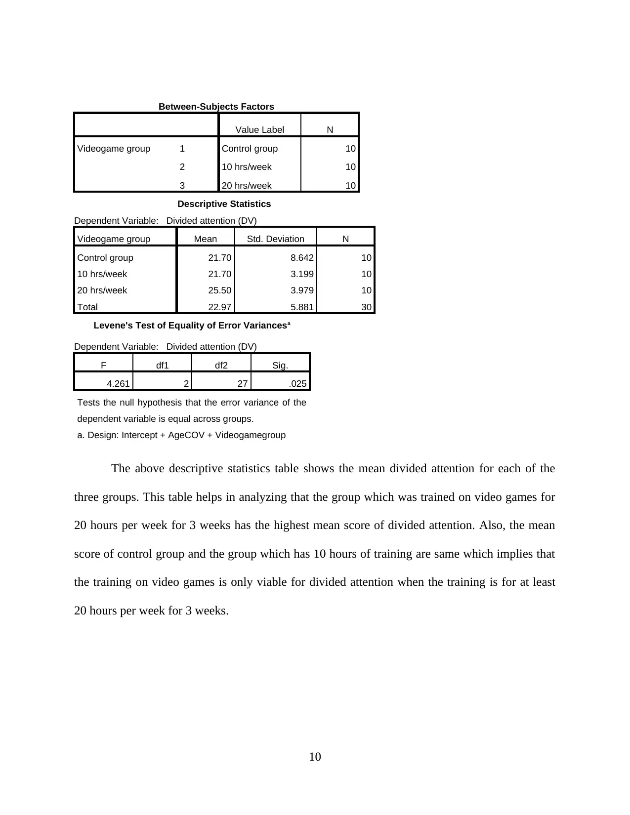
Between-Subjects Factors
Value Label N
Videogame group 1 Control group 10
2 10 hrs/week 10
3 20 hrs/week 10
Descriptive Statistics
Dependent Variable: Divided attention (DV)
Videogame group Mean Std. Deviation N
Control group 21.70 8.642 10
10 hrs/week 21.70 3.199 10
20 hrs/week 25.50 3.979 10
Total 22.97 5.881 30
Levene's Test of Equality of Error Variancesa
Dependent Variable: Divided attention (DV)
F df1 df2 Sig.
4.261 2 27 .025
Tests the null hypothesis that the error variance of the
dependent variable is equal across groups.
a. Design: Intercept + AgeCOV + Videogamegroup
The above descriptive statistics table shows the mean divided attention for each of the
three groups. This table helps in analyzing that the group which was trained on video games for
20 hours per week for 3 weeks has the highest mean score of divided attention. Also, the mean
score of control group and the group which has 10 hours of training are same which implies that
the training on video games is only viable for divided attention when the training is for at least
20 hours per week for 3 weeks.
10
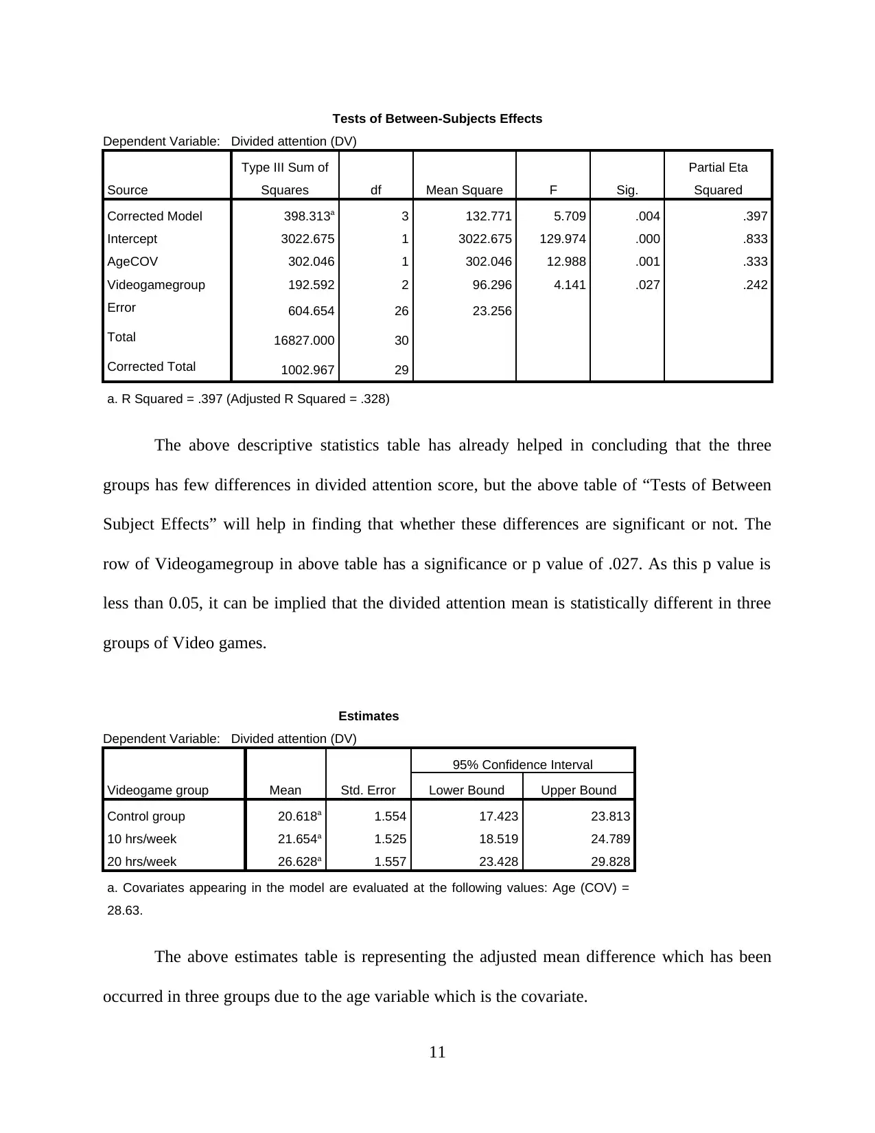
Tests of Between-Subjects Effects
Dependent Variable: Divided attention (DV)
Source
Type III Sum of
Squares df Mean Square F Sig.
Partial Eta
Squared
Corrected Model 398.313a 3 132.771 5.709 .004 .397
Intercept 3022.675 1 3022.675 129.974 .000 .833
AgeCOV 302.046 1 302.046 12.988 .001 .333
Videogamegroup 192.592 2 96.296 4.141 .027 .242
Error 604.654 26 23.256
Total 16827.000 30
Corrected Total 1002.967 29
a. R Squared = .397 (Adjusted R Squared = .328)
The above descriptive statistics table has already helped in concluding that the three
groups has few differences in divided attention score, but the above table of “Tests of Between
Subject Effects” will help in finding that whether these differences are significant or not. The
row of Videogamegroup in above table has a significance or p value of .027. As this p value is
less than 0.05, it can be implied that the divided attention mean is statistically different in three
groups of Video games.
Estimates
Dependent Variable: Divided attention (DV)
Videogame group Mean Std. Error
95% Confidence Interval
Lower Bound Upper Bound
Control group 20.618a 1.554 17.423 23.813
10 hrs/week 21.654a 1.525 18.519 24.789
20 hrs/week 26.628a 1.557 23.428 29.828
a. Covariates appearing in the model are evaluated at the following values: Age (COV) =
28.63.
The above estimates table is representing the adjusted mean difference which has been
occurred in three groups due to the age variable which is the covariate.
11
Dependent Variable: Divided attention (DV)
Source
Type III Sum of
Squares df Mean Square F Sig.
Partial Eta
Squared
Corrected Model 398.313a 3 132.771 5.709 .004 .397
Intercept 3022.675 1 3022.675 129.974 .000 .833
AgeCOV 302.046 1 302.046 12.988 .001 .333
Videogamegroup 192.592 2 96.296 4.141 .027 .242
Error 604.654 26 23.256
Total 16827.000 30
Corrected Total 1002.967 29
a. R Squared = .397 (Adjusted R Squared = .328)
The above descriptive statistics table has already helped in concluding that the three
groups has few differences in divided attention score, but the above table of “Tests of Between
Subject Effects” will help in finding that whether these differences are significant or not. The
row of Videogamegroup in above table has a significance or p value of .027. As this p value is
less than 0.05, it can be implied that the divided attention mean is statistically different in three
groups of Video games.
Estimates
Dependent Variable: Divided attention (DV)
Videogame group Mean Std. Error
95% Confidence Interval
Lower Bound Upper Bound
Control group 20.618a 1.554 17.423 23.813
10 hrs/week 21.654a 1.525 18.519 24.789
20 hrs/week 26.628a 1.557 23.428 29.828
a. Covariates appearing in the model are evaluated at the following values: Age (COV) =
28.63.
The above estimates table is representing the adjusted mean difference which has been
occurred in three groups due to the age variable which is the covariate.
11
⊘ This is a preview!⊘
Do you want full access?
Subscribe today to unlock all pages.
Trusted by 1+ million students worldwide
1 out of 33
Related Documents


Your All-in-One AI-Powered Toolkit for Academic Success.
+13062052269
info@desklib.com
Available 24*7 on WhatsApp / Email
![[object Object]](/_next/static/media/star-bottom.7253800d.svg)
Unlock your academic potential
Copyright © 2020–2026 A2Z Services. All Rights Reserved. Developed and managed by ZUCOL.