SPSS Data Analysis Assignment for PSY 87540: Statistical Analysis

This assignment involves analyzing a dataset using SPSS to answer a series of questions related to psychological and statistical concepts. The questions cover a range of statistical techniques, including calculating descriptive statistics (mean, median, percentages), performing t-tests (one-sample and independent samples), conducting ANOVA (one-way and two-way), calculating correlations, and performing chi-square tests. The analysis explores relationships between variables such as income, marital status, gender, age, lifestyle scores, financial comfort, and relationship happiness. The assignment also involves interpreting the results of these statistical tests and drawing conclusions about the relationships between the variables. The data used in the assignment were collected from a sample of 400 participants in romantic relationships, and the solutions provide detailed answers to each question, including the correct statistical results and interpretations.

QUESTIONS 1-13
Use SPSS and the data file found in syllabus resources (DATA540.SAV) to answer the
following questions. Round your answers to the nearest dollar, percentage point, or whole
number.
#1. What is the mean annual income (INC1) of the participants?
A.$43,282
B.$72,133
C.$47,113
D. $34,282
Answer: (c) $ 47,113
#2 What percent of the participants are married (RELAT)?
a. 28%
b. 33%
c. 51%
d. 59%
Answer: (d) 59%
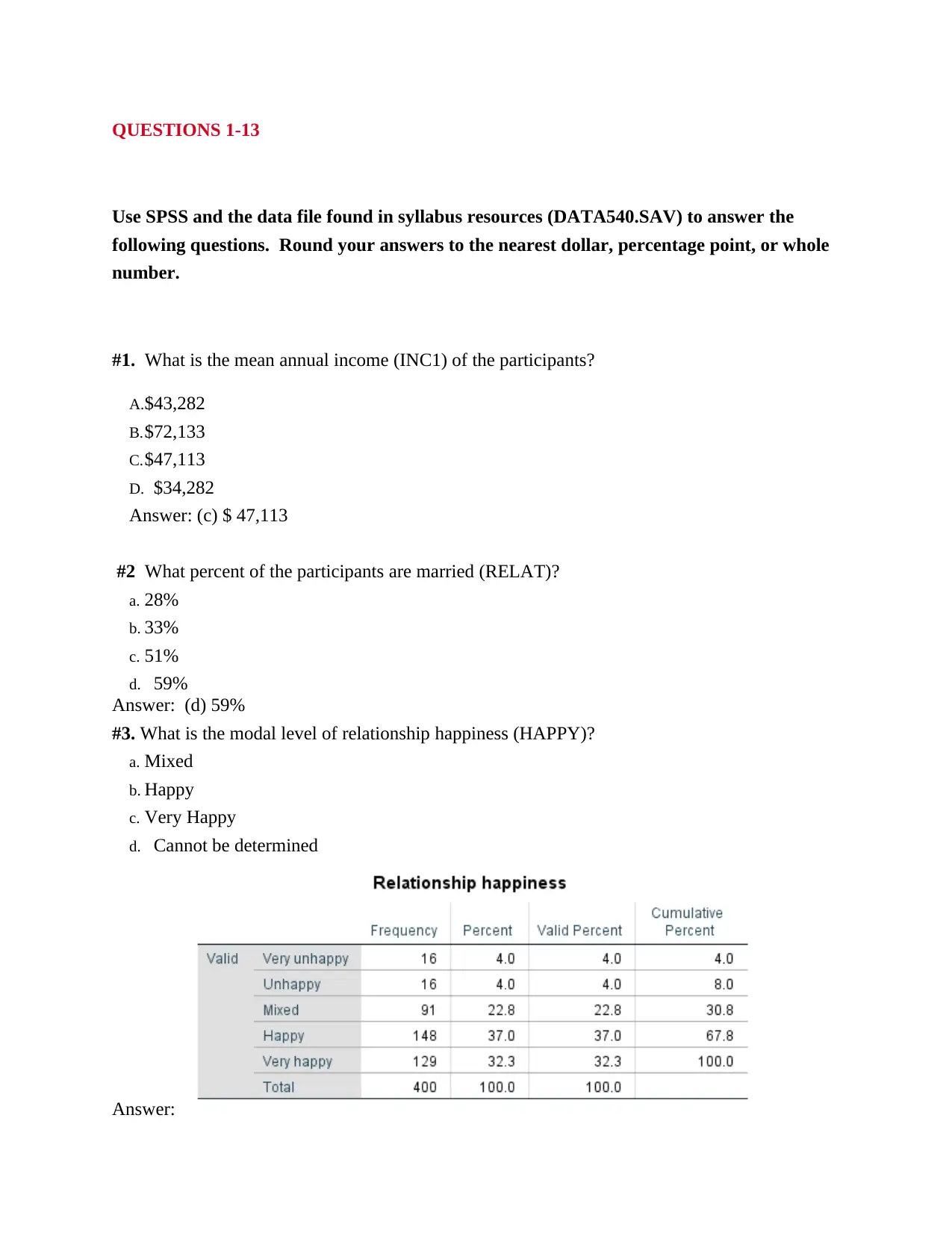
#3. What is the modal level of relationship happiness (HAPPY)?
a. Mixed
b. Happy
c. Very Happy
d. Cannot be determined
Answer:

(b) Happy
#4. What is the median income of the participants’ partners (INC2)?
a. $24,212
b. $28,945
c. $32,000
d. $48,975
Answer: (c) $ 32,000
#5. What percent of the participants are age 51 or older?
a. 4%
b. 5%
c. 7%
d. 10%
Answer: (b) 5%
#6. Test the age of the participants (AGE1) against the null hypothesis H0 = 34. Use a one-
sample t-test. How would you report the results?
a. t = -1.862, df = 399, p > .05
b. t = -1.862, df = 399, p < .05
c. t = 1.645, df = 399, p > .05
d. t = 1.645, df = 399, p < .05
Answer (a) t = -1.862, df = 399, p > .05
#7. What is the mean and standard deviation for the Lifestyle score (L)?
a. 31.22, 7.99
b. 36.19, 8.54
c. 30.03, 7.28
d. 55, 13
Answer: (a) 31.22, 7.99
#8. The first case shown in the data file is a firefighter with a financial Risk-Taking score (R) of
38. What is his Risk-Taking z-score (hint: you will need to find the Risk-Taking mean and
standard deviation)?
a. 0.179
b. -0.223
c. 1.342
d. -1.223

Answer: (a) 0.179
#9. Perform independent sample t-tests on the Lifestyle, Dependency, and Risk-Taking scores
(L, D, and R) comparing men and women (GENDER1). Use p < .05 as your alpha level and
apply a two-tailed test. On each of the three scales, do men or women have a significantly higher
score?
a. Lifestyle: Men, Dependency: Women, Risk-Taking: Men.
b. Lifestyle: Not significantly different, Dependency: Women, Risk-Taking: Men
c. Lifestyle: Women, Dependency: Women, Risk-Taking: Men
d. Lifestyle: Men, Dependency: Men, Risk-Taking: Not significantly different
Answer (b) Lifestyle: Not significantly different, Dependency: Women, Risk-Taking: Men
#10. The median US salary is $50,700, according to US Census data. Using a one-sample t-test,
test to see if participant income (INC1) is different from the national average. Use a two-tailed
test and an alpha level of 5%.
a. Participant income is significantly greater than the national average
b. Participant income is significantly less than the national average
c. Participant income is not significantly different from the national average
d. Participant income cannot be compared to the national average
Answer: (c) participant income is not significantly different from the national average.
#11. Test to see if there is a significant difference between the age of the participant and the age
of the partner. Use a paired-sample t-test and an alpha level of 1%. How would you interpret
the results of this test?
a. The partners are significantly older than the participants.
b. The partners are significantly younger than the participants.
c. The age of the participants and partners are not significantly different.
d. Sometimes the partners are older, sometimes the participants are older.
Answer The partners are significantly older than the participants.
#12. What is the 95% confidence interval for the difference between participant and partner age?
a. The partner is from .60 to 1.76 years older than the participant
b. The participant is from .60 to 1.76 years older than the partner
c. The partner is from 5.88 to 9.45 years older than the participant
d. The participant is from 5.88 to 9.45 years older than the partner
Answer: (a) The partner is from .60 to 1.76 years older than the participant

13. Perform a one-way ANOVA to look at whether income (INC1) differs by type of
relationship (RELAT). Which of the following describes your result:
A. F(3,396) = 4.91, p > .05
B. F(3,396) = 4.91, p < .001
C. F(3,396) = 6.85, p > .05
D. F(3,396) = 6.85, p < .001
Answer: (a) F(3,396) = 4.91, p > .05
QUESTIONS 14-16
______________________________________________________________________
Perform a 2-way ANOVA with participant’s income (INC1) as the dependent variable and with
gender (GENDER1) and marital status (MSTAT) as independent variables. Interpret your
results in questions 14, 15 and 16. (Hint: click the “Plots” button in the Univariate routine
to create a graph).
#14. The main effect due to gender indicates that:
A. Women earn more than men.
B. Men earn more than women.
C. Men and women have incomes that are not significantly different.
D. Participants earn more than their partners.
Answer (b) Men earn more than women.
QUESTIONS 15-26
Use SPSS and the data file found in syllabus resources (DATA540.SAV) to answer the
following questions. Round your answers to the nearest dollar, percentage point, or whole
number.
#15. The main effect due to marital status indicates:
A. Your income tends to decrease after a divorce.
B. Getting married tends to increase your income.
C. Marital status is unrelated to income.
D. Married people tend to earn more than single people.
Answer (d) Married people tend to earn more than single people.

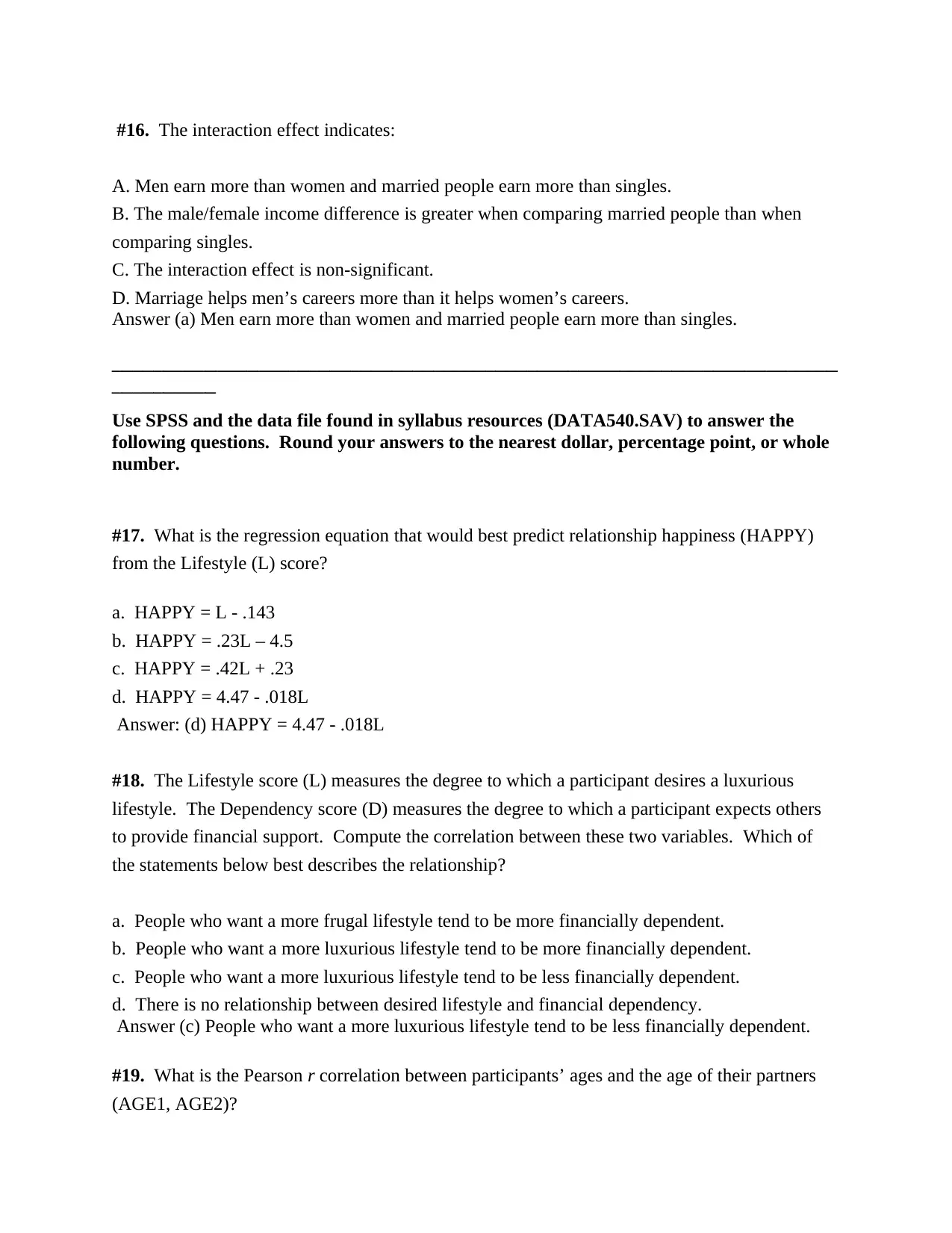
#16. The interaction effect indicates:
A. Men earn more than women and married people earn more than singles.
B. The male/female income difference is greater when comparing married people than when
comparing singles.
C. The interaction effect is non-significant.
D. Marriage helps men’s careers more than it helps women’s careers.
Answer (a) Men earn more than women and married people earn more than singles.
______________________________________________________________________
__________
Use SPSS and the data file found in syllabus resources (DATA540.SAV) to answer the
following questions. Round your answers to the nearest dollar, percentage point, or whole
number.
#17. What is the regression equation that would best predict relationship happiness (HAPPY)
from the Lifestyle (L) score?
a. HAPPY = L - .143
b. HAPPY = .23L – 4.5
c. HAPPY = .42L + .23
d. HAPPY = 4.47 - .018L
Answer: (d) HAPPY = 4.47 - .018L
#18. The Lifestyle score (L) measures the degree to which a participant desires a luxurious
lifestyle. The Dependency score (D) measures the degree to which a participant expects others
to provide financial support. Compute the correlation between these two variables. Which of
the statements below best describes the relationship?
a. People who want a more frugal lifestyle tend to be more financially dependent.
b. People who want a more luxurious lifestyle tend to be more financially dependent.
c. People who want a more luxurious lifestyle tend to be less financially dependent.
d. There is no relationship between desired lifestyle and financial dependency.
Answer (c) People who want a more luxurious lifestyle tend to be less financially dependent.
#19. What is the Pearson r correlation between participants’ ages and the age of their partners
(AGE1, AGE2)?

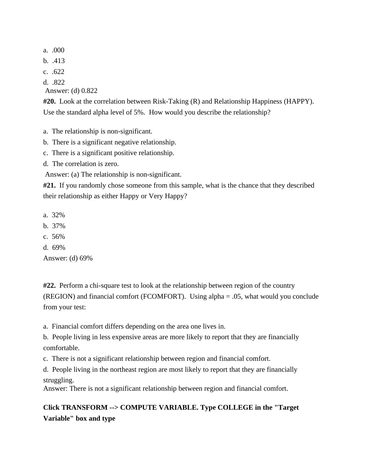
a. .000
b. .413
c. .622
d. .822
Answer: (d) 0.822
#20. Look at the correlation between Risk-Taking (R) and Relationship Happiness (HAPPY).
Use the standard alpha level of 5%. How would you describe the relationship?
a. The relationship is non-significant.
b. There is a significant negative relationship.
c. There is a significant positive relationship.
d. The correlation is zero.
Answer: (a) The relationship is non-significant.
#21. If you randomly chose someone from this sample, what is the chance that they described
their relationship as either Happy or Very Happy?
a. 32%
b. 37%
c. 56%
d. 69%
Answer: (d) 69%
#22. Perform a chi-square test to look at the relationship between region of the country
(REGION) and financial comfort (FCOMFORT). Using alpha = .05, what would you conclude
from your test:
a. Financial comfort differs depending on the area one lives in.
b. People living in less expensive areas are more likely to report that they are financially
comfortable.
c. There is not a significant relationship between region and financial comfort.
d. People living in the northeast region are most likely to report that they are financially
struggling.
Answer: There is not a significant relationship between region and financial comfort.
Click TRANSFORM --> COMPUTE VARIABLE. Type COLLEGE in the "Target
Variable" box and type

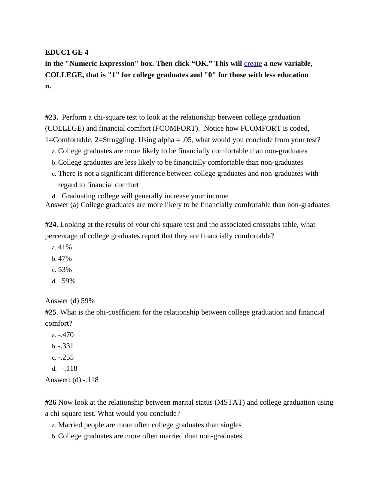
EDUC1 GE 4
in the "Numeric Expression" box. Then click “OK.” This will create a new variable,
COLLEGE, that is "1" for college graduates and "0" for those with less education
n.
#23. Perform a chi-square test to look at the relationship between college graduation
(COLLEGE) and financial comfort (FCOMFORT). Notice how FCOMFORT is coded,
1=Comfortable, 2=Struggling. Using alpha = .05, what would you conclude from your test?
a. College graduates are more likely to be financially comfortable than non-graduates
b. College graduates are less likely to be financially comfortable than non-graduates
c. There is not a significant difference between college graduates and non-graduates with
regard to financial comfort
d. Graduating college will generally increase your income
Answer (a) College graduates are more likely to be financially comfortable than non-graduates
#24. Looking at the results of your chi-square test and the associated crosstabs table, what
percentage of college graduates report that they are financially comfortable?
a. 41%
b. 47%
c. 53%
d. 59%
Answer (d) 59%
#25. What is the phi-coefficient for the relationship between college graduation and financial
comfort?
a. -.470
b. -.331
c. -.255
d. -.118
Answer: (d) -.118
#26 Now look at the relationship between marital status (MSTAT) and college graduation using
a chi-square test. What would you conclude?
a. Married people are more often college graduates than singles
b. College graduates are more often married than non-graduates

c. There is not a significant relationship between marital status and college graduation
d. Both “a” and “b” are true
Answer: (d) Both “a” and “b” are true.