Statistics in Public Health: Quantitative Analysis and Study Review

This report examines the application of statistics in public health, focusing on the analysis of four quantitative peer-reviewed articles related to hypertension and its risk factors. The student explores the role of statistics in identifying population health risks and informing health promotion strategies. T...Read More

Running head: STATISTICS
Statistics
Name of the student:
Name of the Author’s note:
Author’s note

1STATISTICS
Task 1
Statistics is an important analytic tool in the field of public health that aids in health
assessment of a population, identify population at risk and detect new health threats in a
community. Application of statistics has played a crucial role in promoting the translation of data
into causal effect data and identifying risk factors that needs to be addressed by government or
health agency of any specific country (Gleich et al. 2014). Hence, by the identification of
statistics and interpretation of correlation between risk and exposure, it has become possible to
control and manage disease in different settings. This paper will explain the use of statistics in
public health by giving examples of four quantitative peer reviewed articles that explores about
rising incidence of hypertension and its correlation with several risk factors.
Hypertension is a significant public health issue in England as it affects more than one in
England and it is third biggest risk factor for premature death. Preventing hypertension has been
prioritized in UK as it is one of the risk factors of cardiovascular disease and at least one in half
of all heart attacks and strokes have been linked to hypertension. Thus, in order to combat the
burden of hypertension, several researchers have explored the affect or benefit of diet patterns or
lifestyle changes on influencing the rate of hypertension (Public Health England, 2017). The
quantitative study by Lelong et al. (2015) investigated about the relation between nutrition and
blood pressure using a cross-sectional study design. As worldwide guidelines recommend
improvement in lifestyle behaviours for prevention of hypertension, the study aimed to analyse
the influence of dietary intake on blood pressure outcomes (BP). It was a cohort study done with
participants aged above 18 years and data was collected regarding demographics details and
daily dietary intake. The participants had to complete three 24 hours dietary records on three
random days and nutrient intake was estimated using the NutriNet-Santé food composition table.

2STATISTICS
Based on the diet taken, total energy intake was calculated and their dietary questionnaire
provided update on sodium intake from foods. In addition, anthropometrics and blood pressure
measurement was done by trained medical staffs. The significance of the data collection method
is the quality and completeness of dietary investigation which can give high quality estimated on
different nutritional factors and BP.
The significance of the quantitative investigation by Lelong et al. (2015) it used statistical
tools to conclude that salt comsumption has positive relationship with high BP and negative
relationship between fruit and vegetable consumption in preventing hypertension. The study also
reported positive relation between alcohol consumption and hypertension. This conclusion was
possible by the use of descriptive analyses and calculation of Pearson correlation coefficient.
The utility of descriptive analyses is that it helps to calculate standard deviations for each
quantitative variable, thus allowing for simpler interpretation of the data. In addition, Pearson
correlation coefficient is that gave good estimate about the effect size estimate between BP and
different types of food items (Baffoe-Djan and Smith 2019). Thus, statistical analyses helped to
explore correlation between the disease (hypertension) and risk factor (dietary intake) and played
a role in estimating the food item that is most beneficial or harmful for patient with diabetes. As
significant relation between dietary sodium to potassium ratio and BP was found, this study
confirmed that restricting diet intake can reduce or control hypertension.
The study by Aktar (2014) used statistics to explore relation between dietary sodium and
hypertension status based on older adult’s food purchasing and consumption behaviour. The
study was conducted using quantitative survey method and data was collected from 30
community dwelling older adults regarding daily sodium purchased, consumed, DASH score and
DASH dietary pattern. DASH diet is recommended for people with increased risk of developing

3STATISTICS
hypertension. Apart from interview, food receipts and 24 hour recall was also used for data
collection. The quantitative data was analyzed by calculation of frequencies and percentage and
use of independent t-test. The significance of this statistical tool in data analysis was that it
helped to identify statistically significant differences between the groups (Choudhary 2018). All
the statistical analyses were performed in Minitab15 data analysis software which further
enhances the accuracy of the data. From this data analysis, it was found that knowledge about
sodium had no meaningful relationship between among of sodium consumed. Thus, this finding
suggested the need for greater public effort to address intake of sodium in older adults. This
evidence shows how statistics can help to identify the type of public health promotion needed in
response to any disease too.
Two other quantitative research papers have been found that explores relation between
physical activity and hypertension. The study by Xu et al. (2014) explored joint association
between physical activity and hypertension on type 2 diabetes. Two community based
prospective cohort design was used to collect data from adults living in Nanjing, China. For each
participants, physical activity (PA) level and blood pressure status was assessed at baseline and
three years of follow-up and descriptive statistics was used to analyse data for the two studies.
The interaction between PA and hypertension was done using multivariate logistic regression
models. This statistical model is useful in interpreting relation between two or more independent
variables (Faraway 2016). Thus, this study revealed how statistics can be used to explore relation
between multiple variables. Through this form of analysis, the study concluded that sufficient PA
and hypertension can lower the risk of diabetes. In contrast, Moker et al. (2014) utilized statistics
to examine relationship between BP response and exercise training. The study subjects
completed exercise training progeam and the effect of this training on BP response was analyzed

4STATISTICS
using linear and multivariable regression. Use of these statistical methods resulted in ease of
interpretation as estimation of positive or negative effect became easier. Based on statistical
analysis, the study concluded that exercise training may reduce BP. Thus, the above studies
demonstrate various ways in which statistics can explore relation between disease and risk
factors and how they can direct planning appropriate health promotion strategies for target group.
The paper provided a discussion on the application of statistics in public health by
reviewing four quantitative papers explored the relation between lifestyle change and reduction
in BP level. In all the four studies, different variables like diet intake, physical activity, sodium
consumption and exercise was used to interpret the relation between BP and other variables.
These studies used statistical tools like descriptive analyses, regression analysis, correlation
coefficient and t-test to interpret the statistical significance between two or more research
variables. Hence, with such wide role of statistics in public health research, it is necessary that
public health staffs acquire knowledge in statistical tools to interpret recent research works.
Task 2
Case-control study: Case-control study is a type of research design that studies disease pattern
by comparing patients who have a disease (cases) to those patients or groups who do not show
any symptoms of the disease. The aim of this study design is to determine the relationship
between the risk factor and the disease by looking back retrospectively at population at risk of
disease. Unlike randomized controlled trial or experimental studies, no intervention is attempted
in case control studies. It is designed to estimate odds of any disease based on the exposure to the
risk factor of interest. Briefly, it aims to determine if an exposure can lead to an outcome or

5STATISTICS
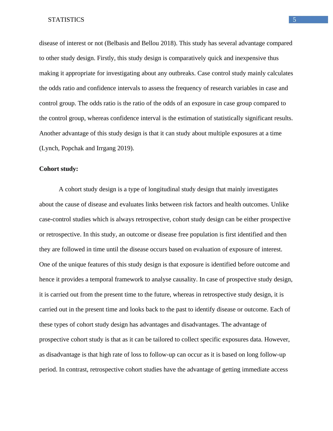
disease of interest or not (Belbasis and Bellou 2018). This study has several advantage compared
to other study design. Firstly, this study design is comparatively quick and inexpensive thus
making it appropriate for investigating about any outbreaks. Case control study mainly calculates
the odds ratio and confidence intervals to assess the frequency of research variables in case and
control group. The odds ratio is the ratio of the odds of an exposure in case group compared to
the control group, whereas confidence interval is the estimation of statistically significant results.
Another advantage of this study design is that it can study about multiple exposures at a time
(Lynch, Popchak and Irrgang 2019).
Cohort study:
A cohort study design is a type of longitudinal study design that mainly investigates
about the cause of disease and evaluates links between risk factors and health outcomes. Unlike
case-control studies which is always retrospective, cohort study design can be either prospective
or retrospective. In this study, an outcome or disease free population is first identified and then
they are followed in time until the disease occurs based on evaluation of exposure of interest.
One of the unique features of this study design is that exposure is identified before outcome and
hence it provides a temporal framework to analyse causality. In case of prospective study design,
it is carried out from the present time to the future, whereas in retrospective study design, it is
carried out in the present time and looks back to the past to identify disease or outcome. Each of
these types of cohort study design has advantages and disadvantages. The advantage of
prospective cohort study is that as it can be tailored to collect specific exposures data. However,
as disadvantage is that high rate of loss to follow-up can occur as it is based on long follow-up
period. In contrast, retrospective cohort studies have the advantage of getting immediate access

6STATISTICS
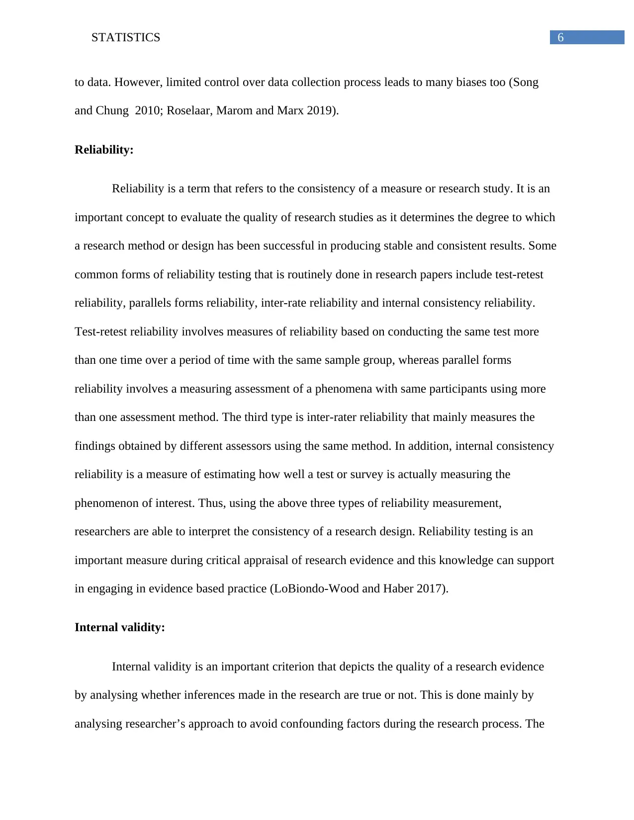
to data. However, limited control over data collection process leads to many biases too (Song
and Chung 2010; Roselaar, Marom and Marx 2019).
Reliability:
Reliability is a term that refers to the consistency of a measure or research study. It is an
important concept to evaluate the quality of research studies as it determines the degree to which
a research method or design has been successful in producing stable and consistent results. Some
common forms of reliability testing that is routinely done in research papers include test-retest
reliability, parallels forms reliability, inter-rate reliability and internal consistency reliability.
Test-retest reliability involves measures of reliability based on conducting the same test more
than one time over a period of time with the same sample group, whereas parallel forms
reliability involves a measuring assessment of a phenomena with same participants using more
than one assessment method. The third type is inter-rater reliability that mainly measures the
findings obtained by different assessors using the same method. In addition, internal consistency
reliability is a measure of estimating how well a test or survey is actually measuring the
phenomenon of interest. Thus, using the above three types of reliability measurement,
researchers are able to interpret the consistency of a research design. Reliability testing is an
important measure during critical appraisal of research evidence and this knowledge can support
in engaging in evidence based practice (LoBiondo-Wood and Haber 2017).
Internal validity:
Internal validity is an important criterion that depicts the quality of a research evidence
by analysing whether inferences made in the research are true or not. This is done mainly by
analysing researcher’s approach to avoid confounding factors during the research process. The

7STATISTICS
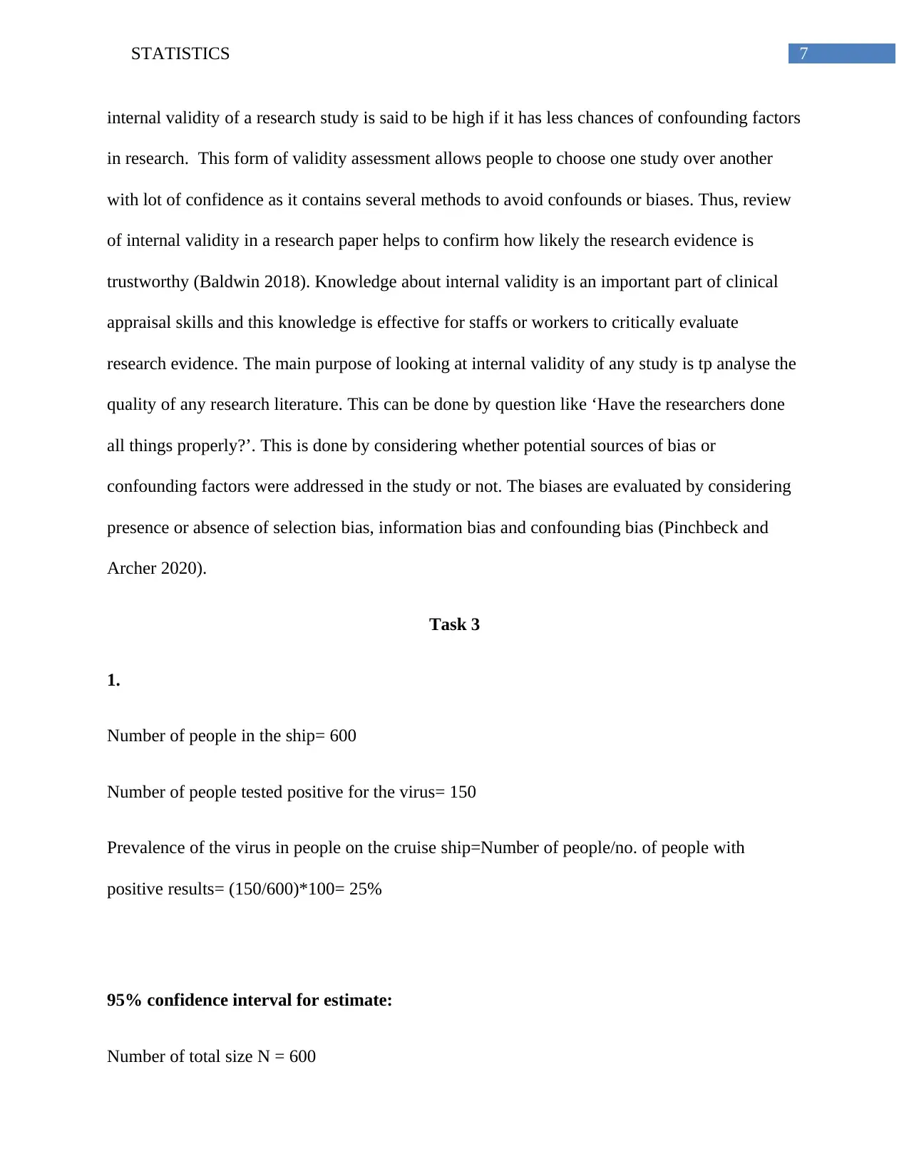
internal validity of a research study is said to be high if it has less chances of confounding factors
in research. This form of validity assessment allows people to choose one study over another
with lot of confidence as it contains several methods to avoid confounds or biases. Thus, review
of internal validity in a research paper helps to confirm how likely the research evidence is
trustworthy (Baldwin 2018). Knowledge about internal validity is an important part of clinical
appraisal skills and this knowledge is effective for staffs or workers to critically evaluate
research evidence. The main purpose of looking at internal validity of any study is tp analyse the
quality of any research literature. This can be done by question like ‘Have the researchers done
all things properly?’. This is done by considering whether potential sources of bias or
confounding factors were addressed in the study or not. The biases are evaluated by considering
presence or absence of selection bias, information bias and confounding bias (Pinchbeck and
Archer 2020).
Task 3
1.
Number of people in the ship= 600
Number of people tested positive for the virus= 150
Prevalence of the virus in people on the cruise ship=Number of people/no. of people with
positive results= (150/600)*100= 25%
95% confidence interval for estimate:
Number of total size N = 600

8STATISTICS
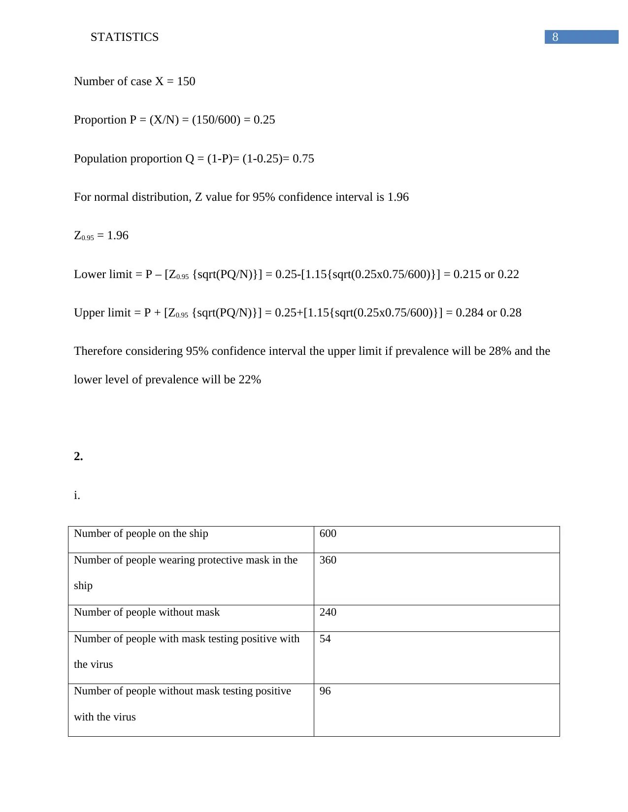
Number of case X = 150
Proportion P = (X/N) = (150/600) = 0.25
Population proportion Q = (1-P)= (1-0.25)= 0.75
For normal distribution, Z value for 95% confidence interval is 1.96
Z0.95 = 1.96
Lower limit = P – [Z0.95 {sqrt(PQ/N)}] = 0.25-[1.15{sqrt(0.25x0.75/600)}] = 0.215 or 0.22
Upper limit = P + [Z0.95 {sqrt(PQ/N)}] = 0.25+[1.15{sqrt(0.25x0.75/600)}] = 0.284 or 0.28
Therefore considering 95% confidence interval the upper limit if prevalence will be 28% and the
lower level of prevalence will be 22%
2.
i.
Number of people on the ship 600
Number of people wearing protective mask in the
ship
360
Number of people without mask 240
Number of people with mask testing positive with
the virus
54
Number of people without mask testing positive
with the virus
96

9STATISTICS
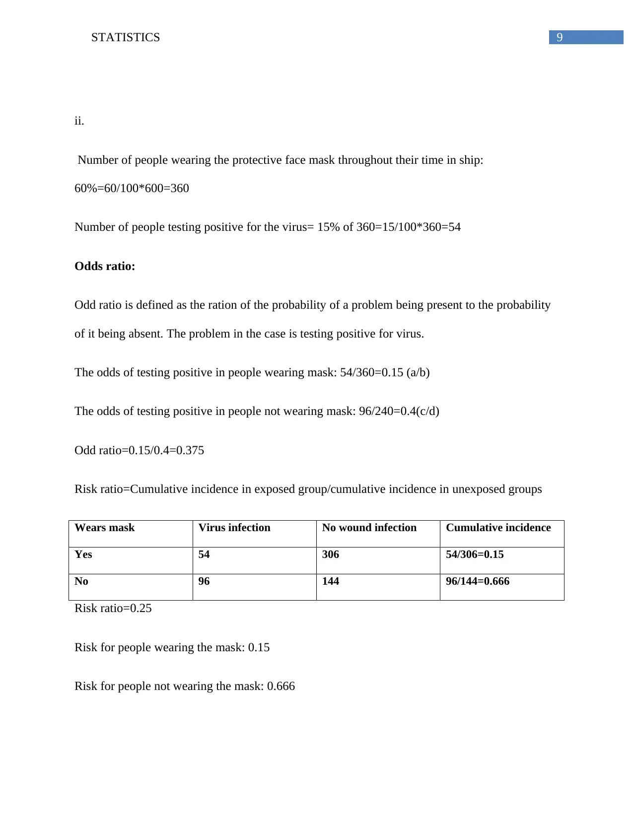
ii.
Number of people wearing the protective face mask throughout their time in ship:
60%=60/100*600=360
Number of people testing positive for the virus= 15% of 360=15/100*360=54
Odds ratio:
Odd ratio is defined as the ration of the probability of a problem being present to the probability
of it being absent. The problem in the case is testing positive for virus.
The odds of testing positive in people wearing mask: 54/360=0.15 (a/b)
The odds of testing positive in people not wearing mask: 96/240=0.4(c/d)
Odd ratio=0.15/0.4=0.375
Risk ratio=Cumulative incidence in exposed group/cumulative incidence in unexposed groups
Wears mask Virus infection No wound infection Cumulative incidence
Yes 54 306 54/306=0.15
No 96 144 96/144=0.666
Risk ratio=0.25
Risk for people wearing the mask: 0.15
Risk for people not wearing the mask: 0.666

10STATISTICS
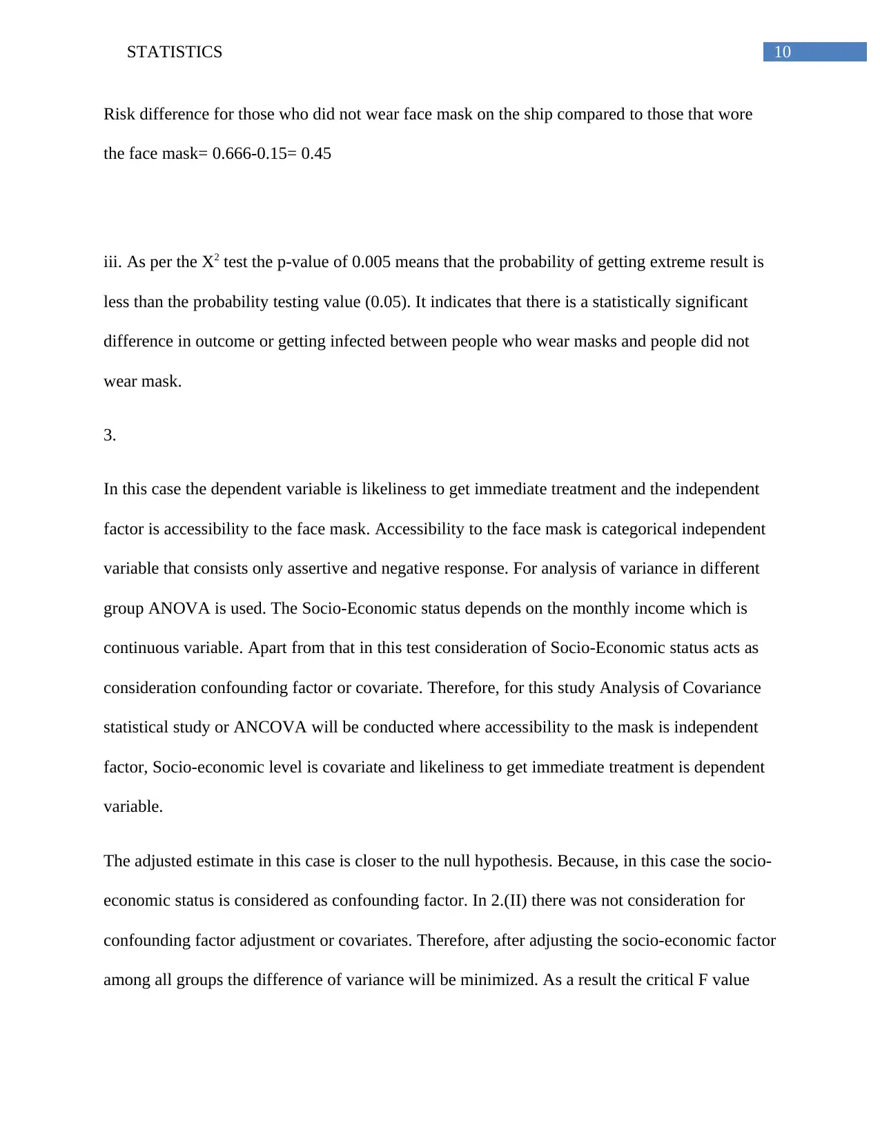
Risk difference for those who did not wear face mask on the ship compared to those that wore
the face mask= 0.666-0.15= 0.45
iii. As per the X2 test the p-value of 0.005 means that the probability of getting extreme result is
less than the probability testing value (0.05). It indicates that there is a statistically significant
difference in outcome or getting infected between people who wear masks and people did not
wear mask.
3.
In this case the dependent variable is likeliness to get immediate treatment and the independent
factor is accessibility to the face mask. Accessibility to the face mask is categorical independent
variable that consists only assertive and negative response. For analysis of variance in different
group ANOVA is used. The Socio-Economic status depends on the monthly income which is
continuous variable. Apart from that in this test consideration of Socio-Economic status acts as
consideration confounding factor or covariate. Therefore, for this study Analysis of Covariance
statistical study or ANCOVA will be conducted where accessibility to the mask is independent
factor, Socio-economic level is covariate and likeliness to get immediate treatment is dependent
variable.
The adjusted estimate in this case is closer to the null hypothesis. Because, in this case the socio-
economic status is considered as confounding factor. In 2.(II) there was not consideration for
confounding factor adjustment or covariates. Therefore, after adjusting the socio-economic factor
among all groups the difference of variance will be minimized. As a result the critical F value

11STATISTICS
will decreased. Henceforth the adjusted estimate be closer to the null hypothesis or further from
null hypothesis than the unadjusted estimate from 2. (II)
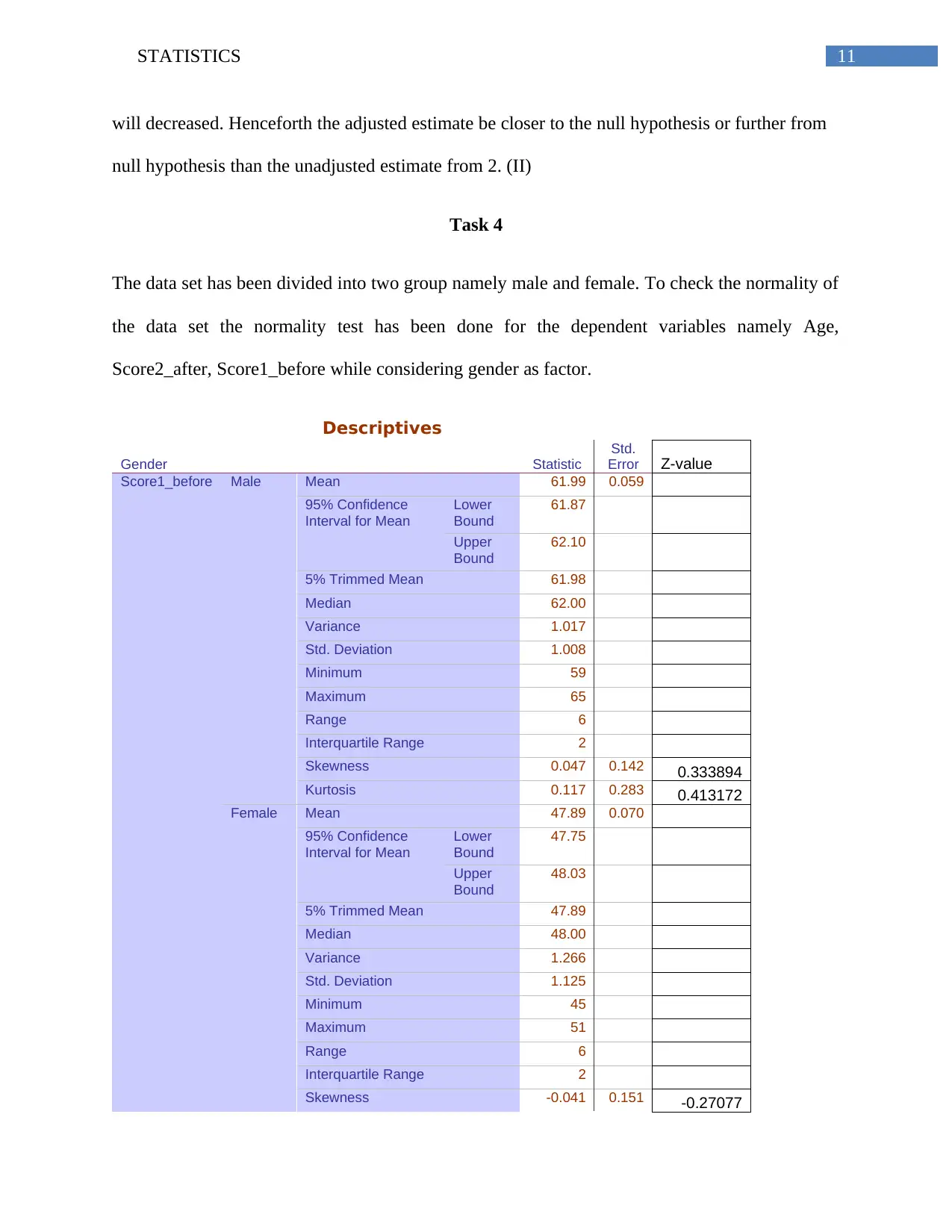
Task 4
The data set has been divided into two group namely male and female. To check the normality of
the data set the normality test has been done for the dependent variables namely Age,
Score2_after, Score1_before while considering gender as factor.
Descriptives
Gender Statistic
Std.
Error Z-value
Score1_before Male Mean 61.99 0.059
95% Confidence
Interval for Mean
Lower
Bound
61.87
Upper
Bound
62.10
5% Trimmed Mean 61.98
Median 62.00
Variance 1.017
Std. Deviation 1.008
Minimum 59
Maximum 65
Range 6
Interquartile Range 2
Skewness 0.047 0.142 0.333894
Kurtosis 0.117 0.283 0.413172
Female Mean 47.89 0.070
95% Confidence
Interval for Mean
Lower
Bound
47.75
Upper
Bound
48.03
5% Trimmed Mean 47.89
Median 48.00
Variance 1.266
Std. Deviation 1.125
Minimum 45
Maximum 51
Range 6
Interquartile Range 2
Skewness -0.041 0.151 -0.27077

12STATISTICS
Kurtosis 0.014 0.301 0.047038
Score2_after Male Mean 74.99 0.060
95% Confidence
Interval for Mean
Lower
Bound
74.88
Upper
Bound
75.11
5% Trimmed Mean 74.99
Median 75.00
Variance 1.044
Std. Deviation 1.022
Minimum 72
Maximum 78
Range 6
Interquartile Range 2
Skewness 0.014 0.142 0.096159
Kurtosis 0.246 0.283 0.869455
Female Mean 65.03 0.061
95% Confidence
Interval for Mean
Lower
Bound
64.91
Upper
Bound
65.15
5% Trimmed Mean 65.04
Median 65.00
Variance 0.953
Std. Deviation 0.976
Minimum 62
Maximum 67
Range 5
Interquartile Range 2
Skewness -0.205 0.151 -1.35523
Kurtosis -0.271 0.301 -0.90065

13STATISTICS
From the normality test by Skewness, Kurtosis and histogram it has been found that the z score
for score1_before and score2_after are greater than -1.96 and less than 1.96. Therefore, the
variables are normally distributed.
Therefore, for the statistical analysis parametric statistical analysis will be used.
Research question 1: Does coffee intake influence test score among University students?
Null hypothesis 1: Test score after is not different from test score before
Alternate hypothesis 1: Test score after is significantly different from test score before
Research Question 2: Is there any association between age and test score (after)?
Null hypothesis 2: Test score after does not depends on age of the participants
Alternate hypothesis 2: Test score after significantly depends on age of the participants
The dataset are parametric and therefore for both cases parametric statistical tests will be used.
To test hypotheses of question 1 the paired t-test analysis will be used. In this case there is a two
group of data where group 1 is the data of test1_before and group 2 is test2_after. Therefore, in
this the analysis of difference in means of two group will be required. Furthermore, the groups

14STATISTICS
are not actually different, rather the data are collected on a same group in two different time.
Hence, Paired T-test will be used.
To test hypotheses of question 2 the regression analysis will be used. Here the age is a
continuous variable and the test2_after is the continuous variable. Therefore to find the
association between two continuous variable regression analysis will be conducted.
Question 1 Hypothesis Test:
Paired Samples Statistics
Mean N Std. Deviation Std. Error Mean
Pair 1 Score1_before 55.37 554 7.122 .303
Score2_after 70.32 554 5.078 .216
Paired Samples Test
Paired Differences
t df
Sig. (2-
tailed)Mean
Std.
Deviation
Std. Error
Mean
95% Confidence Interval
of the Difference
Lower Upper
Pair 1 Score1_before -
Score2_after
-14.946 2.497 .106 -15.154 -14.737 -140.874 553 .000
As per the above analysis significant p value is 0.000 which is less than the probability test value
0.05. Therefore null hypothesis 1 is rejected and alternative hypothesis is accepted. From the
mean values it has been found that Score1_after is larger than Score2_before. Therefore, Test
score after is significantly larger than test score before, which indicates that coffee intake
significantly influences test score among University students.
Question 2 Hypothesis Test:

15STATISTICS
Model Summary
Model R R Square
Adjusted R
Square
Std. Error of the
Estimate
1 .131a .017 .015 5.038
a. Predictors: (Constant), Age
ANOVAa
Model Sum of Squares df Mean Square F Sig.
1 Regression 246.207 1 246.207 9.700 .002b
Residual 14011.513 552 25.383
Total 14257.720 553
a. Dependent Variable: Score2_after
b. Predictors: (Constant), Age
Coefficientsa
Model
Unstandardized Coefficients
Standardized
Coefficients
t Sig.B Std. Error Beta
1 (Constant) 74.384 1.324 56.198 .000
Age -.159 .051 -.131 -3.114 .002
a. Dependent Variable: Score2_after
As per the above analysis of regression through ANOVA and Coefficient analysis it has been
found that in both cases the significance value is 0.002, which is less than the less than the
probability test value 0.05. Therefore null hypothesis 1 is rejected and alternative hypothesis is
accepted. Hence, test score after significantly depends on age of the participants. The t-value is
negative in coefficient test. It indicates that there is an inverse association between age and test
score after. Therefore, with the increase of age the test score after decreases among University
students.

16STATISTICS
References:
Aktar, A., 2014. Dietary Sodium and Hypertension Status: A Quantitative Study Exploring Older
Adults’ Food Purchasing and Consumption Behaviour. Retrieved
from:https://ir.lib.uwo.ca/cgi/viewcontent.cgi?article=3919&context=etd
Baffoe-Djan, J.B. and Smith, S.A., 2019. Descriptive statistics in data analysis. In The Routledge
Handbook of Research Methods in Applied Linguistics (pp. 398-414). Routledge.

17STATISTICS
Baldwin, L., 2018. Internal and External Validity and Threats to Validity. In Research Concepts
for the Practitioner of Educational Leadership (pp. 31-36). Brill Sense.
Belbasis, L. and Bellou, V., 2018. Introduction to epidemiological studies. In Genetic
Epidemiology (pp. 1-6). Humana Press, New York, NY.
Choudhary, R., 2018. Application of “independent t-test” by using SPSS for conducting physical
education researches. Hypothesis, 20(92), p.99.
Faraway, J.J., 2016. Extending the linear model with R: generalized linear, mixed effects and
nonparametric regression models. CRC press.
Gleich, S., Viehöver, S., Teipel, A., Drubba, S., Turlik, V. and Hirl, B., 2019. Death certificates-
an underestimated source of information for statistics, judicature, public health, and
science. Bundesgesundheitsblatt, Gesundheitsforschung, Gesundheitsschutz.
Lelong, H., Galan, P., Kesse-Guyot, E., Fezeu, L., Hercberg, S. and Blacher, J., 2015.
Relationship between nutrition and blood pressure: a cross-sectional analysis from the NutriNet-
Santé Study, a french web-based cohort study. American journal of hypertension, 28(3), pp.362-
371.
LoBiondo-Wood, G. and Haber, J., 2017. Nursing research-E-book: methods and critical
appraisal for evidence-based practice. Elsevier Health Sciences.
Lynch, A.D., Popchak, A.J. and Irrgang, J.J., 2019. Level III Evidence: A Case-Control Study.
In Basic Methods Handbook for Clinical Orthopaedic Research (pp. 295-300). Springer, Berlin,
Heidelberg.

18STATISTICS
Moker, E. A., Bateman, L. A., Kraus, W. E., and Pescatello, L. S. 2014. The relationship
between the blood pressure responses to exercise following training and detraining periods. PloS
one, 9(9).
Pinchbeck, G.L. and Archer, D.C., 2020. How to critically appraise a paper. Equine Veterinary
Education, 32(2), pp.104-109.
Public Health England. (2017). Health matters: combating high blood pressure. Retrieved from:
https://www.gov.uk/government/publications/health-matters-combating-high-blood-pressure/
health-matters-combating-high-blood-pressure
Roselaar, N., Marom, N. and Marx, R.G., 2019. Level 2 Evidence: Prospective Cohort Study.
In Basic Methods Handbook for Clinical Orthopaedic Research (pp. 289-293). Springer, Berlin,
Heidelberg.
Song, J.W. and Chung, K.C., 2010. Observational studies: cohort and case-control
studies. Plastic and reconstructive surgery, 126(6), p.2234
Xu, F., Ware, R.S., Tse, L.A., Wang, Y., Wang, Z., Hong, X., Chan, E.Y.Y., Dunstan, D.W. and
Owen, N., 2014. Joint associations of physical activity and hypertension with the development of
type 2 diabetes among urban men and women in Mainland China. PLoS One, 9(2).

19STATISTICS