Nonlinear Programming Approach to Step-Cone Pulley Optimization

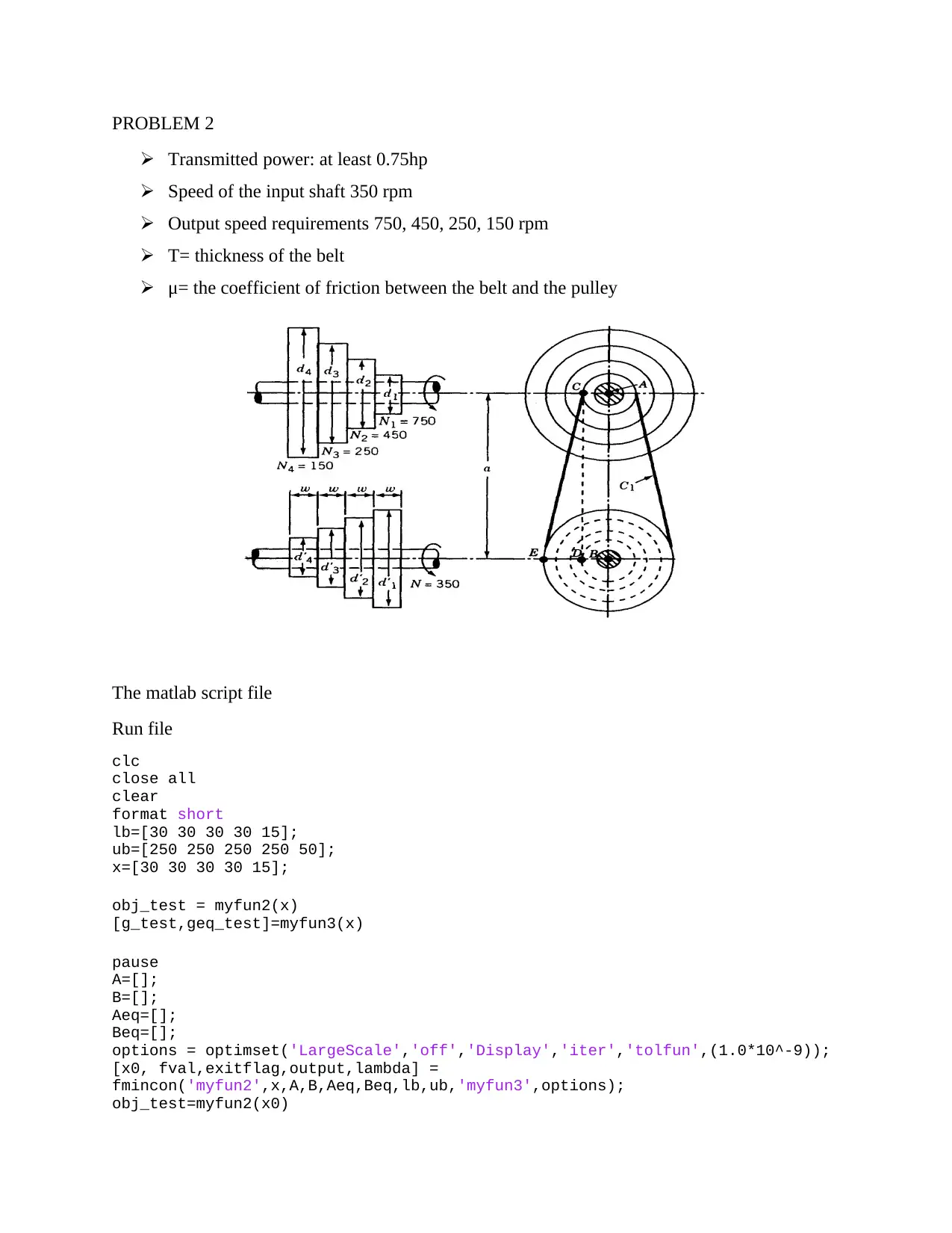
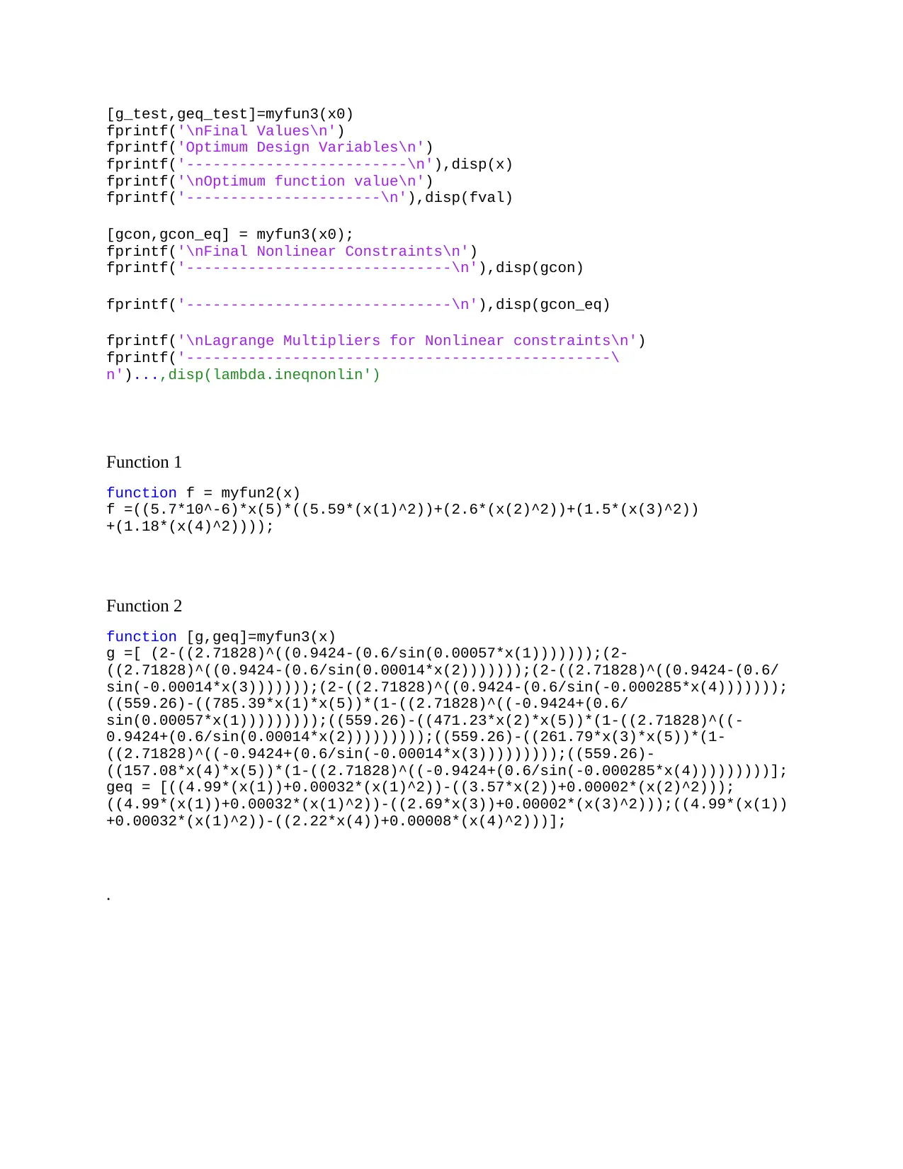
This project focuses on the design optimization of a step-cone pulley using nonlinear programming techniques. The goal is to minimize the weight of the pulley while meeting specific power transmission and speed requirements. The problem is formulated with constraints related to belt tension, output speeds, and other design parameters. The solution involves using MATLAB to implement optimization algorithms, defining objective functions and constraints, and iteratively refining the design variables to achieve an optimal solution. The project report includes detailed design information, discusses the effects of design variables on the pulley's weight, and compares the results obtained from different optimization approaches. This document provides a comprehensive approach to solving a practical engineering problem through numerical optimization, with the aim of creating an efficient and lightweight step-cone pulley system. Desklib provides access to similar solved assignments and past papers for students.

UNIVERSITY AFFILIATION
FACULTY OR DEPARTMENT
COURSE ID & NAME
TITLE: NON-LINEAR PROGRAMMING
STUDENT NAME
STUDENT REGISTRATION NUMBER
PROFESSOR (TUTOR)
DATE OF SUBMISSION
2018

PROBLEM 2
 Transmitted power: at least 0.75hp
 Speed of the input shaft 350 rpm
 Output speed requirements 750, 450, 250, 150 rpm
 T= thickness of the belt
 μ= the coefficient of friction between the belt and the pulley
The matlab script file
Run file
clc
close all
clear
format short
lb=[30 30 30 30 15];
ub=[250 250 250 250 50];
x=[30 30 30 30 15];
obj_test = myfun2(x)
[g_test,geq_test]=myfun3(x)
pause
A=[];
B=[];
Aeq=[];
Beq=[];
options = optimset('LargeScale','off','Display','iter','tolfun',(1.0*10^-9));
[x0, fval,exitflag,output,lambda] =
fmincon('myfun2',x,A,B,Aeq,Beq,lb,ub,'myfun3',options);
obj_test=myfun2(x0)

[g_test,geq_test]=myfun3(x0)
fprintf('\nFinal Values\n')
fprintf('Optimum Design Variables\n')
fprintf('-------------------------\n'),disp(x)
fprintf('\nOptimum function value\n')
fprintf('----------------------\n'),disp(fval)
[gcon,gcon_eq] = myfun3(x0);
fprintf('\nFinal Nonlinear Constraints\n')
fprintf('------------------------------\n'),disp(gcon)
fprintf('------------------------------\n'),disp(gcon_eq)
fprintf('\nLagrange Multipliers for Nonlinear constraints\n')
fprintf('------------------------------------------------\
n')...,disp(lambda.ineqnonlin')
Function 1
function f = myfun2(x)
f =((5.7*10^-6)*x(5)*((5.59*(x(1)^2))+(2.6*(x(2)^2))+(1.5*(x(3)^2))
+(1.18*(x(4)^2))));
Function 2
function [g,geq]=myfun3(x)
g =[ (2-((2.71828)^((0.9424-(0.6/sin(0.00057*x(1)))))));(2-
((2.71828)^((0.9424-(0.6/sin(0.00014*x(2)))))));(2-((2.71828)^((0.9424-(0.6/
sin(-0.00014*x(3)))))));(2-((2.71828)^((0.9424-(0.6/sin(-0.000285*x(4)))))));
((559.26)-((785.39*x(1)*x(5))*(1-((2.71828)^((-0.9424+(0.6/
sin(0.00057*x(1)))))))));((559.26)-((471.23*x(2)*x(5))*(1-((2.71828)^((-
0.9424+(0.6/sin(0.00014*x(2)))))))));((559.26)-((261.79*x(3)*x(5))*(1-
((2.71828)^((-0.9424+(0.6/sin(-0.00014*x(3)))))))));((559.26)-
((157.08*x(4)*x(5))*(1-((2.71828)^((-0.9424+(0.6/sin(-0.000285*x(4)))))))))];
geq = [((4.99*(x(1))+0.00032*(x(1)^2))-((3.57*x(2))+0.00002*(x(2)^2)));
((4.99*(x(1))+0.00032*(x(1)^2))-((2.69*x(3))+0.00002*(x(3)^2)));((4.99*(x(1))
+0.00032*(x(1)^2))-((2.22*x(4))+0.00008*(x(4)^2)))];
.