QAB105: Quantitative Analysis for Business - Semester 2 Assignment

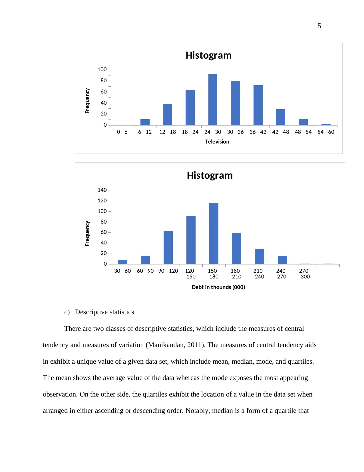
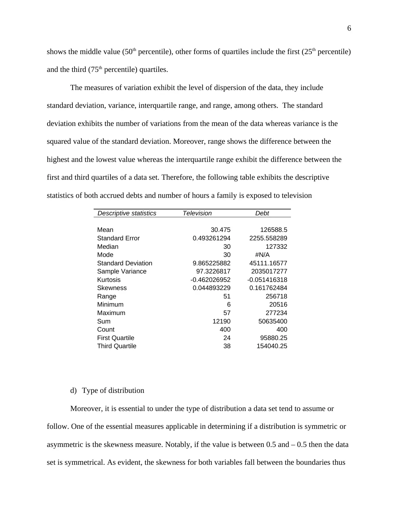
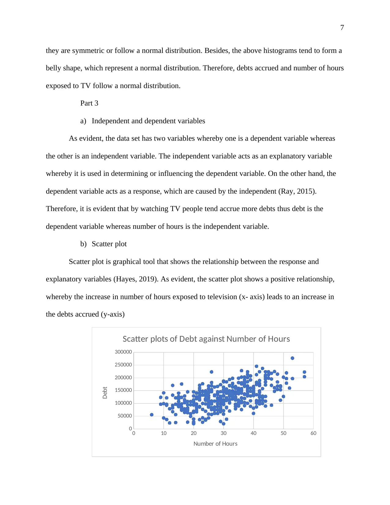
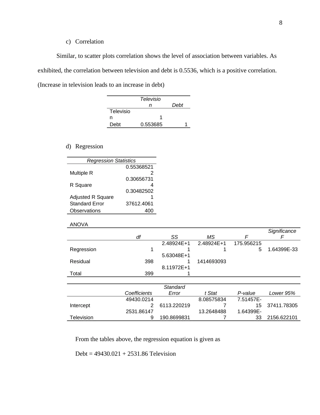
This assignment solution provides a comprehensive quantitative analysis of a business scenario, addressing the relationship between television exposure and family debt. The solution begins by outlining survey methods, specifically focusing on longitudinal cohort surveys, and detailing both probabilistic and non-probabilistic sampling techniques, with a preference for purposive sampling. It then progresses to data analysis, including the creation of class intervals, frequency tables, and histograms for variables such as hours of television watched and family debt. Descriptive statistics, including measures of central tendency (mean, median, mode) and dispersion (standard deviation, variance), are calculated and discussed. The analysis further explores the type of distribution, concluding that both variables follow a normal distribution. The solution identifies independent and dependent variables, constructs a scatter plot to visualize the relationship, and calculates the correlation between television viewing and debt. Finally, it presents a regression analysis, including the regression equation, the fitness of the model (R-squared), and hypothesis testing, concluding that there is a significant relationship between television exposure and accrued debt. The solution is supported by relevant references.

1
Quantitative analysis of business
Name:
Institution:

2
Part 1
a) Type of survey method
Survey is a technique applicable for collecting and compiling data from a group of people
or objects known as a sample (subset of a population). There are three types of survey, which
include cross-sectional, longitudinal, and retrospective surveys (Bhat, 2019). The cross-sectional
surveys are administered to a small sample from a larger population within a limited time frame.
Notably, the cross-sectional survey offers a researcher an opportunity to summarize the opinions
of the respondents at a given time. Longitudinal surveys are applicable in making observation
and collecting of data over an extended period of time. There are three main types of longitudinal
survey, which include, trend, panel, and cohort surveys (Bhat, 2019). Trend surveys are
applicable in determining the shift or transformation in the thought process of respondent over a
period of time whereas panel surveys are administered to the same group of people over the
years. On the other side, cohort surveys are administered to people that meet certain criteria or
characteristics.
The retrospective surveys are administered with an aim of collecting data from past
events. Therefore, among the above surveys the moat appropriate type of survey for collecting
the data is the longitudinal survey, specifically the cohort survey. As evident, the sociologist
hypothesized people who watch television frequently are exposed to many commercials tend to
buy the products, which results in debt. Thus, the study will only administer the survey to people
who watch or own a television set (criteria or characteristics of the respondent).
b) Sampling method
There are two main method of sampling, which include the probabilistic and non-
probabilistic sampling methods (Singh, 2018). The probabilistic sampling uses the randomization

3
to ensure that all elements of the population have an equal chance of being selected in the
sample. They include simple random, stratified, systematic, cluster, and multi-stage sampling.
On the other side, non-probabilistic sampling does not use randomization rather the method
relies on the researcher’s ability to select elements for the sample. They include convenience,
purposeful, quota, and snowball sampling. Notably, the main purpose of the study is to exhibit
the relationship between the number of hours families are exposed to watching television and the
debts accrued by the family. Therefore, the appropriate method of sampling is the non-
probabilistic, specifically purposive sampling since the elements will be selected from the
population which suits the purpose of the study.
c) Challenges of the methods
However, there are various challenges expected during data collection, which include
biasness and influences beyond the control of the researcher; besides, the study may experience
high level of sampling error.
Part 2
a) Class intervals
As evident, both the number of hours exposed to television and debt have 10 class
intervals. The class intervals are given by diving the highest-class size boundary by the class
size.
i. Number of hours exposed to television per week
Highest class size limit = 60
Class size = 6
Number of class size = 60 / 6 = 10

4
The following table exhibit the class intervals and sizes for the number of hours the
television is turned on per week.
Television
Frequen
cy
0 - 6 1
6 - 12 11
12 - 18 38
18 - 24 63
24 - 30 92
30 - 36 80
36 - 42 72
42 - 48 29
48 - 54 12
54- 60 2
ii. Debts per family
Highest class size limit = 300000
Class size =30000
Number of class size = 300000 / 30000 = 10
The following table exhibit the class intervals and sizes for the total debt per family in
thousand dollars ($000)
Debt
Frequenc
y
0 - 30 8
30 - 60 16
60 - 90 63
90 - 120 91
120 - 150 116
150 - 180 59
180 - 210 29
210 - 240 16
240 - 270 1
270 - 300 1
b) Histogram
Histogram is graphical tool that exhibits the distribution of a variable thus the following
histograms show the distribution of both debt and number of hours the television is turned on.

5
0 - 6 6 - 12 12 - 18 18 - 24 24 - 30 30 - 36 36 - 42 42 - 48 48 - 54 54 - 60
0
20
40
60
80
100
Histogram
Television
Frequency
30 - 60 60 - 90 90 - 120 120 -
150 150 -
180 180 -
210 210 -
240 240 -
270 270 -
300
0
20
40
60
80
100
120
140
Histogram
Debt in thounds (000)
Frequency
c) Descriptive statistics
There are two classes of descriptive statistics, which include the measures of central
tendency and measures of variation (Manikandan, 2011). The measures of central tendency aids
in exhibit a unique value of a given data set, which include mean, median, mode, and quartiles.
The mean shows the average value of the data whereas the mode exposes the most appearing
observation. On the other side, the quartiles exhibit the location of a value in the data set when
arranged in either ascending or descending order. Notably, median is a form of a quartile that

6
shows the middle value (50th percentile), other forms of quartiles include the first (25th percentile)
and the third (75th percentile) quartiles.
The measures of variation exhibit the level of dispersion of the data, they include
standard deviation, variance, interquartile range, and range, among others. The standard
deviation exhibits the number of variations from the mean of the data whereas variance is the
squared value of the standard deviation. Moreover, range shows the difference between the
highest and the lowest value whereas the interquartile range exhibit the difference between the
first and third quartiles of a data set. Therefore, the following table exhibits the descriptive
statistics of both accrued debts and number of hours a family is exposed to television
Descriptive statistics Television Debt
Mean 30.475 126588.5
Standard Error 0.493261294 2255.558289
Median 30 127332
Mode 30 #N/A
Standard Deviation 9.865225882 45111.16577
Sample Variance 97.3226817 2035017277
Kurtosis -0.462026952 -0.051416318
Skewness 0.044893229 0.161762484
Range 51 256718
Minimum 6 20516
Maximum 57 277234
Sum 12190 50635400
Count 400 400
First Quartile 24 95880.25
Third Quartile 38 154040.25
d) Type of distribution
Moreover, it is essential to under the type of distribution a data set tend to assume or
follow. One of the essential measures applicable in determining if a distribution is symmetric or
asymmetric is the skewness measure. Notably, if the value is between 0.5 and – 0.5 then the data
set is symmetrical. As evident, the skewness for both variables fall between the boundaries thus

7
they are symmetric or follow a normal distribution. Besides, the above histograms tend to form a
belly shape, which represent a normal distribution. Therefore, debts accrued and number of hours
exposed to TV follow a normal distribution.
Part 3
a) Independent and dependent variables
As evident, the data set has two variables whereby one is a dependent variable whereas
the other is an independent variable. The independent variable acts as an explanatory variable
whereby it is used in determining or influencing the dependent variable. On the other hand, the
dependent variable acts as a response, which are caused by the independent (Ray, 2015).
Therefore, it is evident that by watching TV people tend accrue more debts thus debt is the
dependent variable whereas number of hours is the independent variable.
b) Scatter plot
Scatter plot is graphical tool that shows the relationship between the response and
explanatory variables (Hayes, 2019). As evident, the scatter plot shows a positive relationship,
whereby the increase in number of hours exposed to television (x- axis) leads to an increase in
the debts accrued (y-axis)
0 10 20 30 40 50 60
0
50000
100000
150000
200000
250000
300000
Scatter plots of Debt against Number of Hours
Number of Hours
Debt

8
c) Correlation
Similar, to scatter plots correlation shows the level of association between variables. As
exhibited, the correlation between television and debt is 0.5536, which is a positive correlation.
(Increase in television leads to an increase in debt)
Televisio
n Debt
Televisio
n 1
Debt 0.553685 1
d) Regression
Regression Statistics
Multiple R
0.55368521
2
R Square
0.30656731
4
Adjusted R Square
0.30482502
1
Standard Error 37612.4061
Observations 400
ANOVA
df SS MS F
Significance
F
Regression 1
2.48924E+1
1
2.48924E+1
1
175.956215
5 1.64399E-33
Residual 398
5.63048E+1
1 1414693093
Total 399
8.11972E+1
1
Coefficients
Standard
Error t Stat P-value Lower 95%
Intercept
49430.0214
2 6113.220219
8.08575834
7
7.51457E-
15 37411.78305
Television
2531.86147
9 190.8699831
13.2648488
7
1.64399E-
33 2156.622101
From the tables above, the regression equation is given as
Debt = 49430.021 + 2531.86 Television

9
It is exhibited that the mean response of the families is $49430.021, whereby despite
watching or not each family has a debt of approximately $49430.021. Besides, a unit increase in
the number of hours watch television leads to an increase debt by $2531.86
e) Fitness of the model
As shown, the R square value of the regression is 0.3066, which exhibits that the
variation in debt is explained by exposure to television at the rate of 30.66%. Therefore, the
model is 30.66% fit in explaining accrued debt in each family.
f) Hypothesis
Since the P-value 1.64399E-33 is less than the significance level (0.05) it is evident that
the model is adequate and we conclude that there is a relationship between the number of hours a
family is exposed to watching television and the debt accrued by the respective family.
Part 4
The results above indicate that exposure to TV dependent variable whereas number of
hours is the independent variable. Moreover, both the scatter plot and the correlation measure
show a positive relationship, whereby the increase in number of hours exposed to leads to an
increase in the debts accrued. Consequently, the R square value of 0.3066, which exhibits that
the model is 30.66% fit in explaining accrued debt in each family. Similarly, since the P-value
1.64399E-33 is less than the significance level (0.05) it is evident that the model is adequate and
we conclude that there is a relationship. Therefore, the study concludes the hypothesis by the
sociologist that people who watch television frequently are exposed to many adverts, which
result in increased debt.

10
References
Bhat, A. (2019). Types of Survey with Examples. Retrieved from QuestionPro Website:
https://www.questionpro.com/blog/types-of-survey/
Hayes, A. (2019, June 2019). Correlation Retrieved from Investopedia Website:
https://www.investopedia.com/terms/c/correlation.asp
Manikandan, S. (2011). Measures of central tendency: The mean. Journal of Pharmacol &
Pharmacotherapeutics, 140-142. doi:10.4103/0976-500X.81920
Ray, S. (2015, August 14). Regression Techniques. Retrieved from Analytics Vidhya Website:
https://www.analyticsvidhya.com/blog/2015/08/comprehensive-guide-regression/
Singh, S. (2018, July 26). Sampling Techniques. Retrieved from Towards Data Science Website:
https://towardsdatascience.com/sampling-techniques-a4e34111d808