QMUL BUSM112: Data Analysis Assignment, Applied Economic Methods

This document presents a comprehensive solution to a data assignment for the BUSM112 module, focusing on applied economic methods. The assignment is divided into four parts (A-D), each addressing specific aspects of data analysis and interpretation. Part A analyzes the characteristics of treatment and placebo groups, examining differences in age, exam scores, assets, and size, along with statistical significance. Part B delves into difference-in-differences estimators, evaluating the impact of a treatment on earnings. Part C explores instrumental variables, assessing the reliability of results and endogeneity. Finally, Part D investigates the concepts of stationary and non-stationary time series, analyzing exchange rates. The solution includes relevant tables, regression outputs, and the syntax used to replicate the results, providing a complete and detailed analysis of the data and its implications.

Applied empirical methods
1
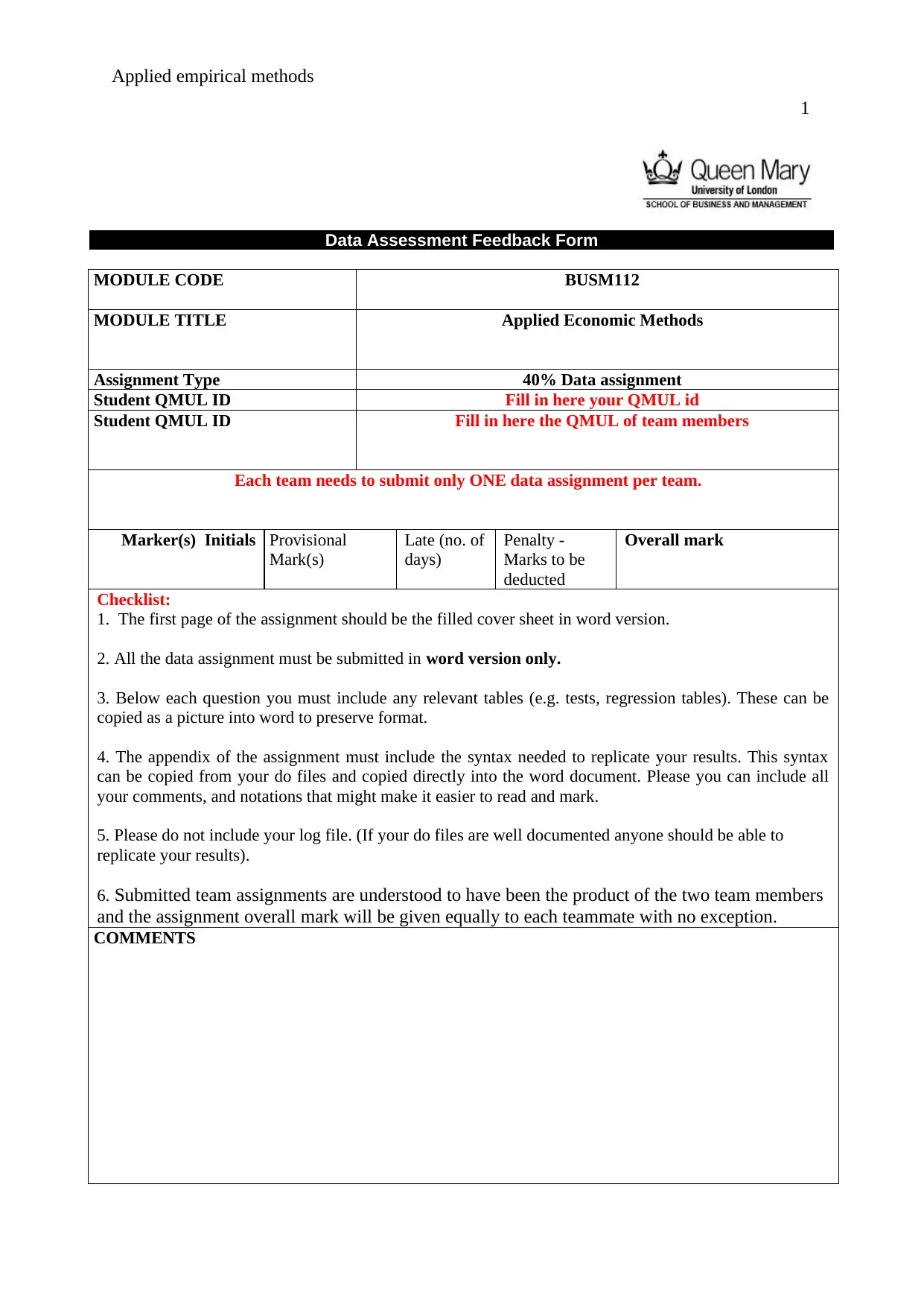
Data Assessment Feedback Form
MODULE CODE BUSM112
MODULE TITLE Applied Economic Methods
Assignment Type 40% Data assignment
Student QMUL ID Fill in here your QMUL id
Student QMUL ID Fill in here the QMUL of team members
Each team needs to submit only ONE data assignment per team.
Marker(s) Initials Provisional
Mark(s)
Late (no. of
days)
Penalty -
Marks to be
deducted
Overall mark
Checklist:
1. The first page of the assignment should be the filled cover sheet in word version.
2. All the data assignment must be submitted in word version only.
3. Below each question you must include any relevant tables (e.g. tests, regression tables). These can be
copied as a picture into word to preserve format.
4. The appendix of the assignment must include the syntax needed to replicate your results. This syntax
can be copied from your do files and copied directly into the word document. Please you can include all
your comments, and notations that might make it easier to read and mark.
5. Please do not include your log file. (If your do files are well documented anyone should be able to
replicate your results).
6. Submitted team assignments are understood to have been the product of the two team members
and the assignment overall mark will be given equally to each teammate with no exception.
COMMENTS

Applied empirical methods
2
Part A [30 Marks]
Quiz (a)
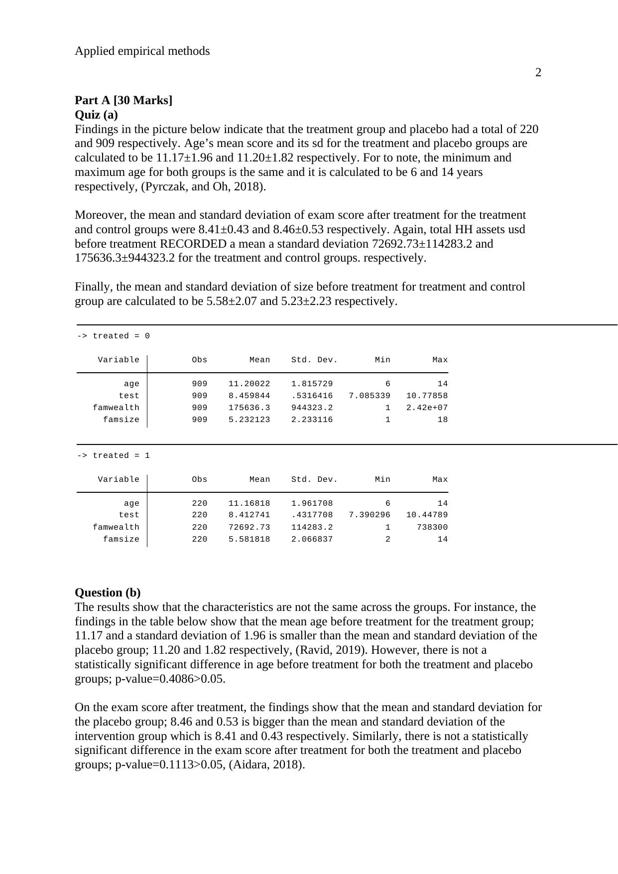
Findings in the picture below indicate that the treatment group and placebo had a total of 220
and 909 respectively. Age’s mean score and its sd for the treatment and placebo groups are
calculated to be 11.17±1.96 and 11.20±1.82 respectively. For to note, the minimum and
maximum age for both groups is the same and it is calculated to be 6 and 14 years
respectively, (Pyrczak, and Oh, 2018).
Moreover, the mean and standard deviation of exam score after treatment for the treatment
and control groups were 8.41±0.43 and 8.46±0.53 respectively. Again, total HH assets usd
before treatment RECORDED a mean a standard deviation 72692.73±114283.2 and
175636.3±944323.2 for the treatment and control groups. respectively.
Finally, the mean and standard deviation of size before treatment for treatment and control
group are calculated to be 5.58±2.07 and 5.23±2.23 respectively.
famsize 220 5.581818 2.066837 2 14
famwealth 220 72692.73 114283.2 1 738300
test 220 8.412741 .4317708 7.390296 10.44789
age 220 11.16818 1.961708 6 14
Variable Obs Mean Std. Dev. Min Max
-> treated = 1
famsize 909 5.232123 2.233116 1 18
famwealth 909 175636.3 944323.2 1 2.42e+07
test 909 8.459844 .5316416 7.085339 10.77858
age 909 11.20022 1.815729 6 14
Variable Obs Mean Std. Dev. Min Max
-> treated = 0
Question (b)
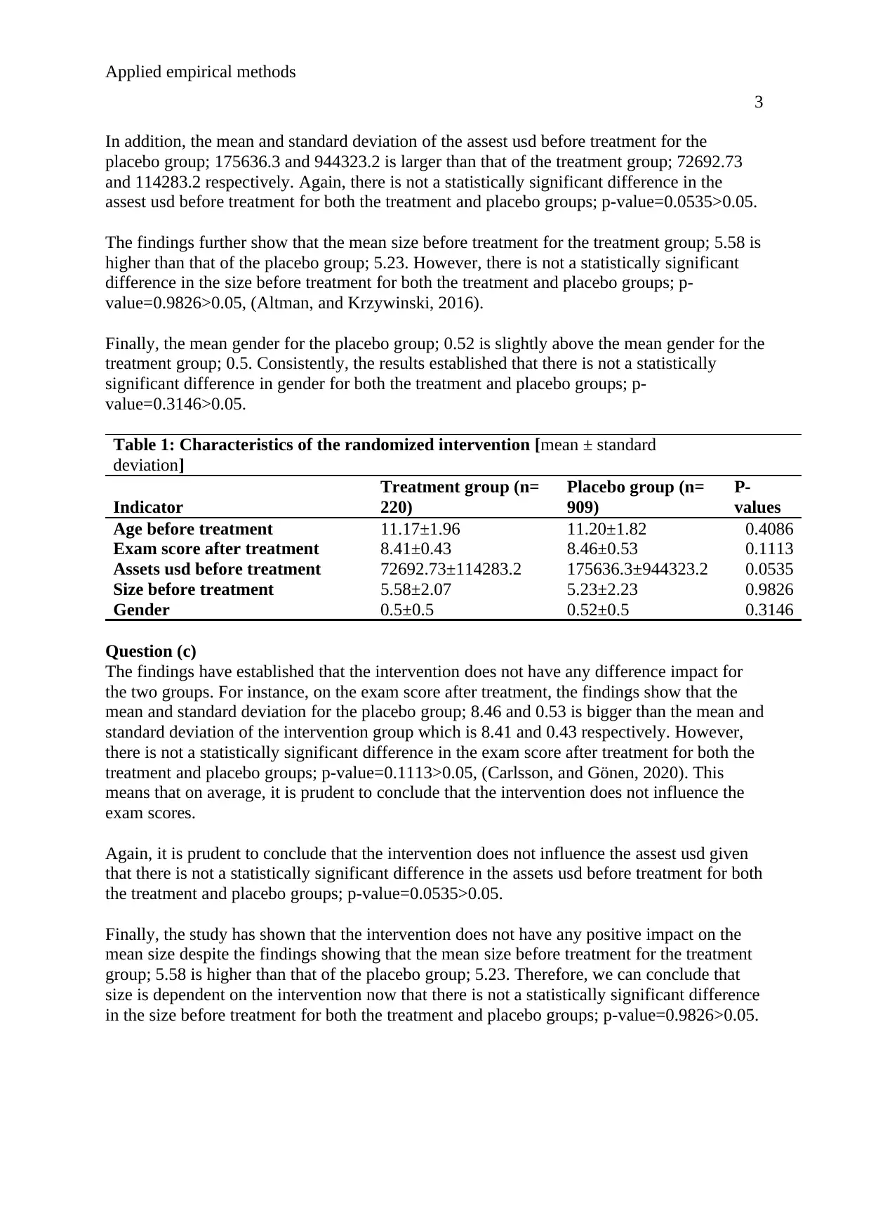
The results show that the characteristics are not the same across the groups. For instance, the
findings in the table below show that the mean age before treatment for the treatment group;
11.17 and a standard deviation of 1.96 is smaller than the mean and standard deviation of the
placebo group; 11.20 and 1.82 respectively, (Ravid, 2019). However, there is not a
statistically significant difference in age before treatment for both the treatment and placebo
groups; p-value=0.4086>0.05.
On the exam score after treatment, the findings show that the mean and standard deviation for
the placebo group; 8.46 and 0.53 is bigger than the mean and standard deviation of the
intervention group which is 8.41 and 0.43 respectively. Similarly, there is not a statistically
significant difference in the exam score after treatment for both the treatment and placebo
groups; p-value=0.1113>0.05, (Aidara, 2018).

Applied empirical methods
3
In addition, the mean and standard deviation of the assest usd before treatment for the
placebo group; 175636.3 and 944323.2 is larger than that of the treatment group; 72692.73
and 114283.2 respectively. Again, there is not a statistically significant difference in the
assest usd before treatment for both the treatment and placebo groups; p-value=0.0535>0.05.
The findings further show that the mean size before treatment for the treatment group; 5.58 is
higher than that of the placebo group; 5.23. However, there is not a statistically significant
difference in the size before treatment for both the treatment and placebo groups; p-
value=0.9826>0.05, (Altman, and Krzywinski, 2016).
Finally, the mean gender for the placebo group; 0.52 is slightly above the mean gender for the
treatment group; 0.5. Consistently, the results established that there is not a statistically
significant difference in gender for both the treatment and placebo groups; p-
value=0.3146>0.05.
Table 1: Characteristics of the randomized intervention [mean ± standard
deviation]
Indicator
Treatment group (n=
220)
Placebo group (n=
909)
P-
values
Age before treatment 11.17±1.96 11.20±1.82 0.4086
Exam score after treatment 8.41±0.43 8.46±0.53 0.1113
Assets usd before treatment 72692.73±114283.2 175636.3±944323.2 0.0535
Size before treatment 5.58±2.07 5.23±2.23 0.9826
Gender 0.5±0.5 0.52±0.5 0.3146
Question (c)
The findings have established that the intervention does not have any difference impact for
the two groups. For instance, on the exam score after treatment, the findings show that the
mean and standard deviation for the placebo group; 8.46 and 0.53 is bigger than the mean and
standard deviation of the intervention group which is 8.41 and 0.43 respectively. However,
there is not a statistically significant difference in the exam score after treatment for both the
treatment and placebo groups; p-value=0.1113>0.05, (Carlsson, and Gönen, 2020). This
means that on average, it is prudent to conclude that the intervention does not influence the
exam scores.
Again, it is prudent to conclude that the intervention does not influence the assest usd given
that there is not a statistically significant difference in the assets usd before treatment for both
the treatment and placebo groups; p-value=0.0535>0.05.
Finally, the study has shown that the intervention does not have any positive impact on the
mean size despite the findings showing that the mean size before treatment for the treatment
group; 5.58 is higher than that of the placebo group; 5.23. Therefore, we can conclude that
size is dependent on the intervention now that there is not a statistically significant difference
in the size before treatment for both the treatment and placebo groups; p-value=0.9826>0.05.

Applied empirical methods
4
Question (d)
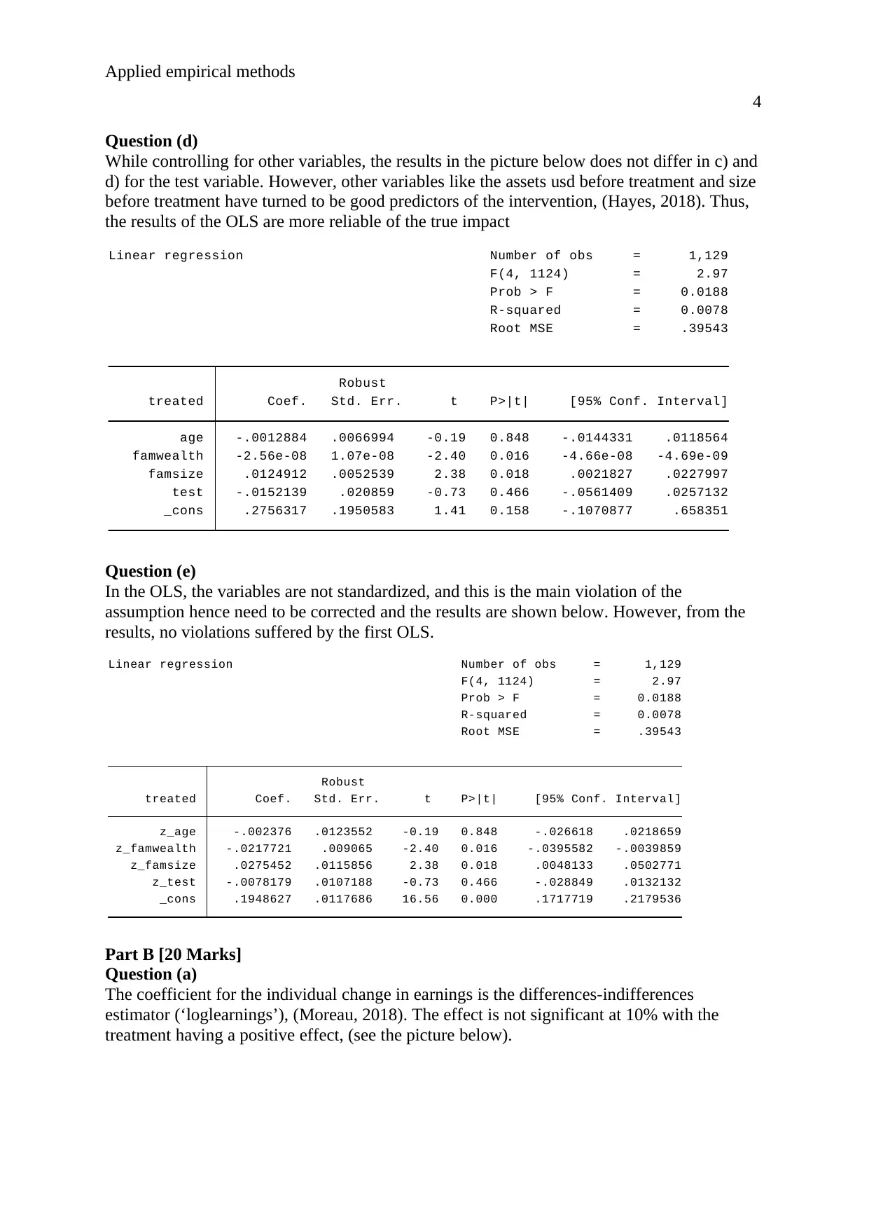
While controlling for other variables, the results in the picture below does not differ in c) and
d) for the test variable. However, other variables like the assets usd before treatment and size
before treatment have turned to be good predictors of the intervention, (Hayes, 2018). Thus,
the results of the OLS are more reliable of the true impact
_cons .2756317 .1950583 1.41 0.158 -.1070877 .658351
test -.0152139 .020859 -0.73 0.466 -.0561409 .0257132
famsize .0124912 .0052539 2.38 0.018 .0021827 .0227997
famwealth -2.56e-08 1.07e-08 -2.40 0.016 -4.66e-08 -4.69e-09
age -.0012884 .0066994 -0.19 0.848 -.0144331 .0118564
treated Coef. Std. Err. t P>|t| [95% Conf. Interval]
Robust
Root MSE = .39543
R-squared = 0.0078
Prob > F = 0.0188
F(4, 1124) = 2.97
Linear regression Number of obs = 1,129
Question (e)
In the OLS, the variables are not standardized, and this is the main violation of the
assumption hence need to be corrected and the results are shown below. However, from the
results, no violations suffered by the first OLS.
_cons .1948627 .0117686 16.56 0.000 .1717719 .2179536
z_test -.0078179 .0107188 -0.73 0.466 -.028849 .0132132
z_famsize .0275452 .0115856 2.38 0.018 .0048133 .0502771
z_famwealth -.0217721 .009065 -2.40 0.016 -.0395582 -.0039859
z_age -.002376 .0123552 -0.19 0.848 -.026618 .0218659
treated Coef. Std. Err. t P>|t| [95% Conf. Interval]
Robust
Root MSE = .39543
R-squared = 0.0078
Prob > F = 0.0188
F(4, 1124) = 2.97
Linear regression Number of obs = 1,129
Part B [20 Marks]
Question (a)
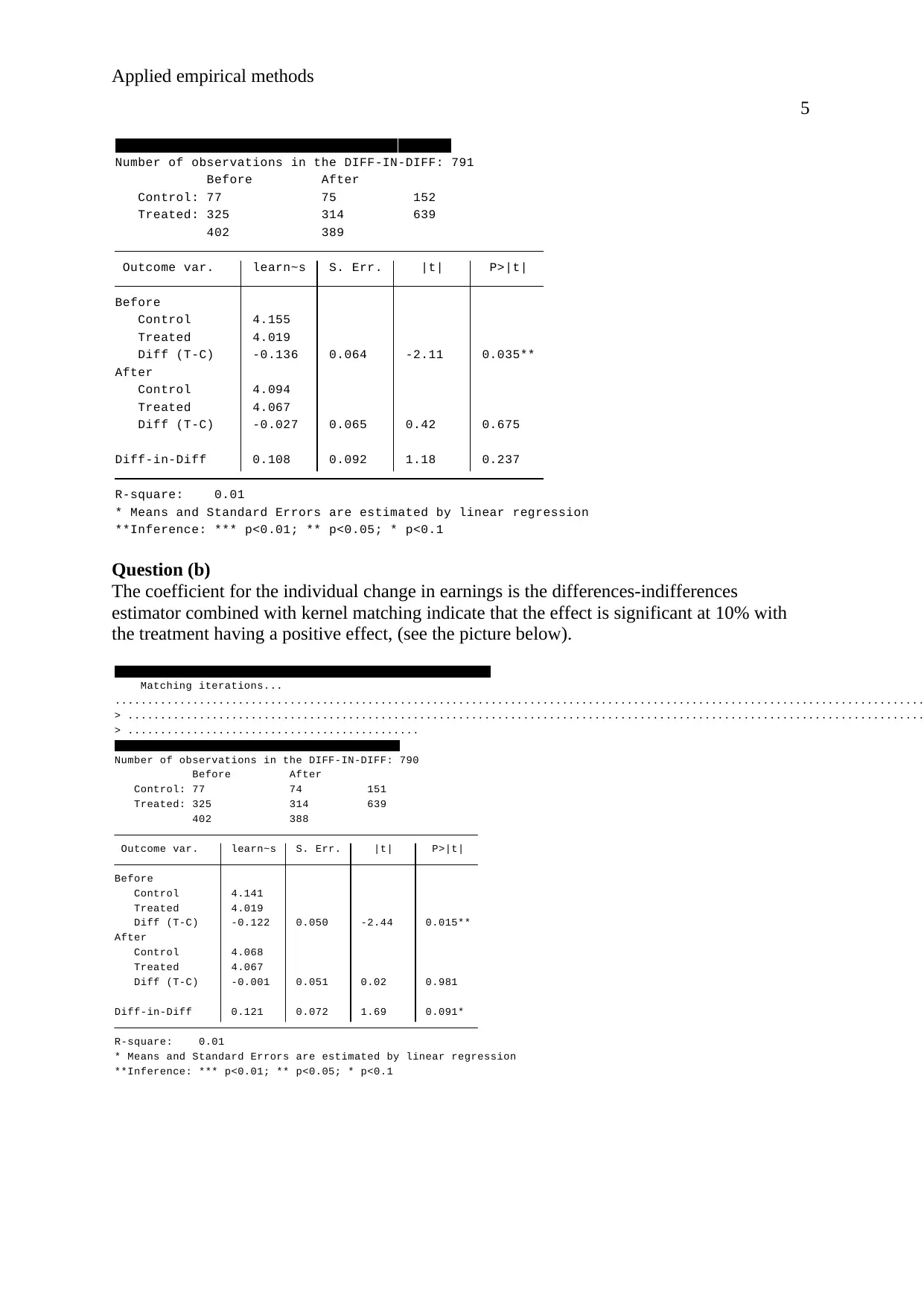
The coefficient for the individual change in earnings is the differences-indifferences
estimator (‘loglearnings’), (Moreau, 2018). The effect is not significant at 10% with the
treatment having a positive effect, (see the picture below).

Applied empirical methods
5
**Inference: *** p<0.01; ** p<0.05; * p<0.1
* Means and Standard Errors are estimated by linear regression
R-square: 0.01
Diff-in-Diff 0.108 0.092 1.18 0.237
Diff (T-C) -0.027 0.065 0.42 0.675
Treated 4.067
Control 4.094
After
Diff (T-C) -0.136 0.064 -2.11 0.035**
Treated 4.019
Control 4.155
Before
Outcome var. learn~s S. Err. |t| P>|t|
402 389
Treated: 325 314 639
Control: 77 75 152
Before After
Number of observations in the DIFF-IN-DIFF: 791
DIFFERENCE-IN-DIFFERENCES ESTIMATION RESULTS
Question (b)
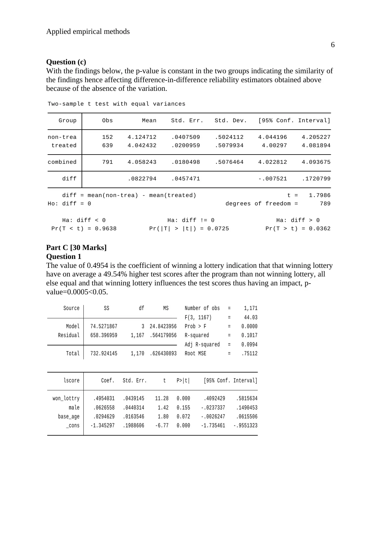
The coefficient for the individual change in earnings is the differences-indifferences
estimator combined with kernel matching indicate that the effect is significant at 10% with
the treatment having a positive effect, (see the picture below).
**Inference: *** p<0.01; ** p<0.05; * p<0.1
* Means and Standard Errors are estimated by linear regression
R-square: 0.01
Diff-in-Diff 0.121 0.072 1.69 0.091*
Diff (T-C) -0.001 0.051 0.02 0.981
Treated 4.067
Control 4.068
After
Diff (T-C) -0.122 0.050 -2.44 0.015**
Treated 4.019
Control 4.141
Before
Outcome var. learn~s S. Err. |t| P>|t|
402 388
Treated: 325 314 639
Control: 77 74 151
Before After
Number of observations in the DIFF-IN-DIFF: 790
DIFFERENCE-IN-DIFFERENCES ESTIMATION RESULTS
> .............................................
> ...........................................................................................................................
.............................................................................................................................
Matching iterations...
KERNEL PROPENSITY SCORE MATCHING DIFFERENCE-IN-DIFFERENCES

Applied empirical methods
6
Question (c)
With the findings below, the p-value is constant in the two groups indicating the similarity of
the findings hence affecting difference-in-difference reliability estimators obtained above
because of the absence of the variation.
Pr(T < t) = 0.9638 Pr(|T| > |t|) = 0.0725 Pr(T > t) = 0.0362
Ha: diff < 0 Ha: diff != 0 Ha: diff > 0
Ho: diff = 0 degrees of freedom = 789
diff = mean(non-trea) - mean(treated) t = 1.7986
diff .0822794 .0457471 -.007521 .1720799
combined 791 4.058243 .0180498 .5076464 4.022812 4.093675
treated 639 4.042432 .0200959 .5079934 4.00297 4.081894
non-trea 152 4.124712 .0407509 .5024112 4.044196 4.205227
Group Obs Mean Std. Err. Std. Dev. [95% Conf. Interval]
Two-sample t test with equal variances
Part C [30 Marks]
Question 1
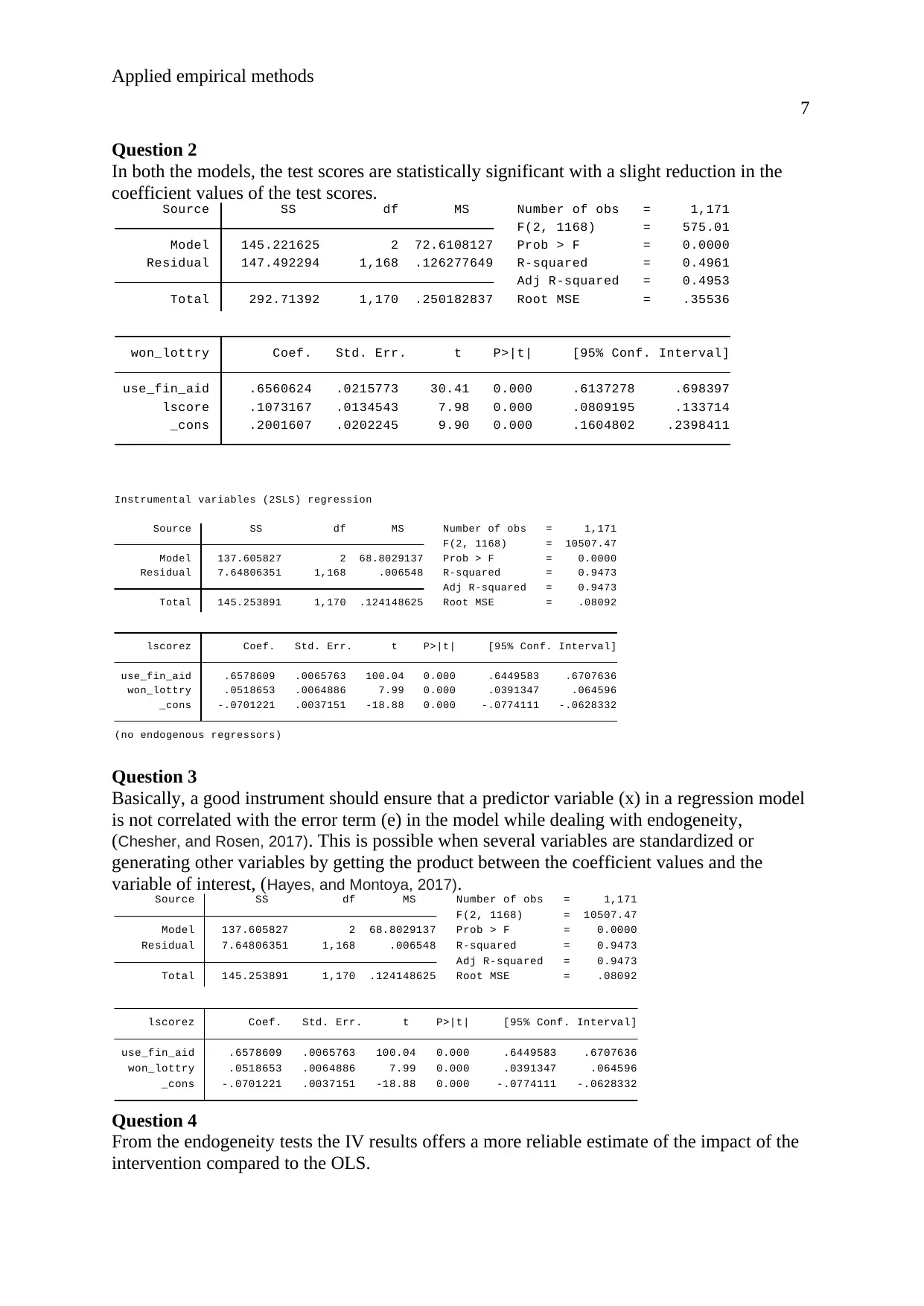
The value of 0.4954 is the coefficient of winning a lottery indication that that winning lottery
have on average a 49.54% higher test scores after the program than not winning lottery, all
else equal and that winning lottery influences the test scores thus having an impact, p-
value=0.0005<0.05.
_cons -1.345297 .1988606 -6.77 0.000 -1.735461 -.9551323
base_age .0294629 .0163546 1.80 0.072 -.0026247 .0615506
male .0626558 .0440314 1.42 0.155 -.0237337 .1490453
won_lottry .4954031 .0439145 11.28 0.000 .4092429 .5815634
lscore Coef. Std. Err. t P>|t| [95% Conf. Interval]
Total 732.924145 1,170 .626430893 Root MSE = .75112
Adj R-squared = 0.0994
Residual 658.396959 1,167 .564179056 R-squared = 0.1017
Model 74.5271867 3 24.8423956 Prob > F = 0.0000
F(3, 1167) = 44.03
Source SS df MS Number of obs = 1,171

Applied empirical methods
7
Question 2
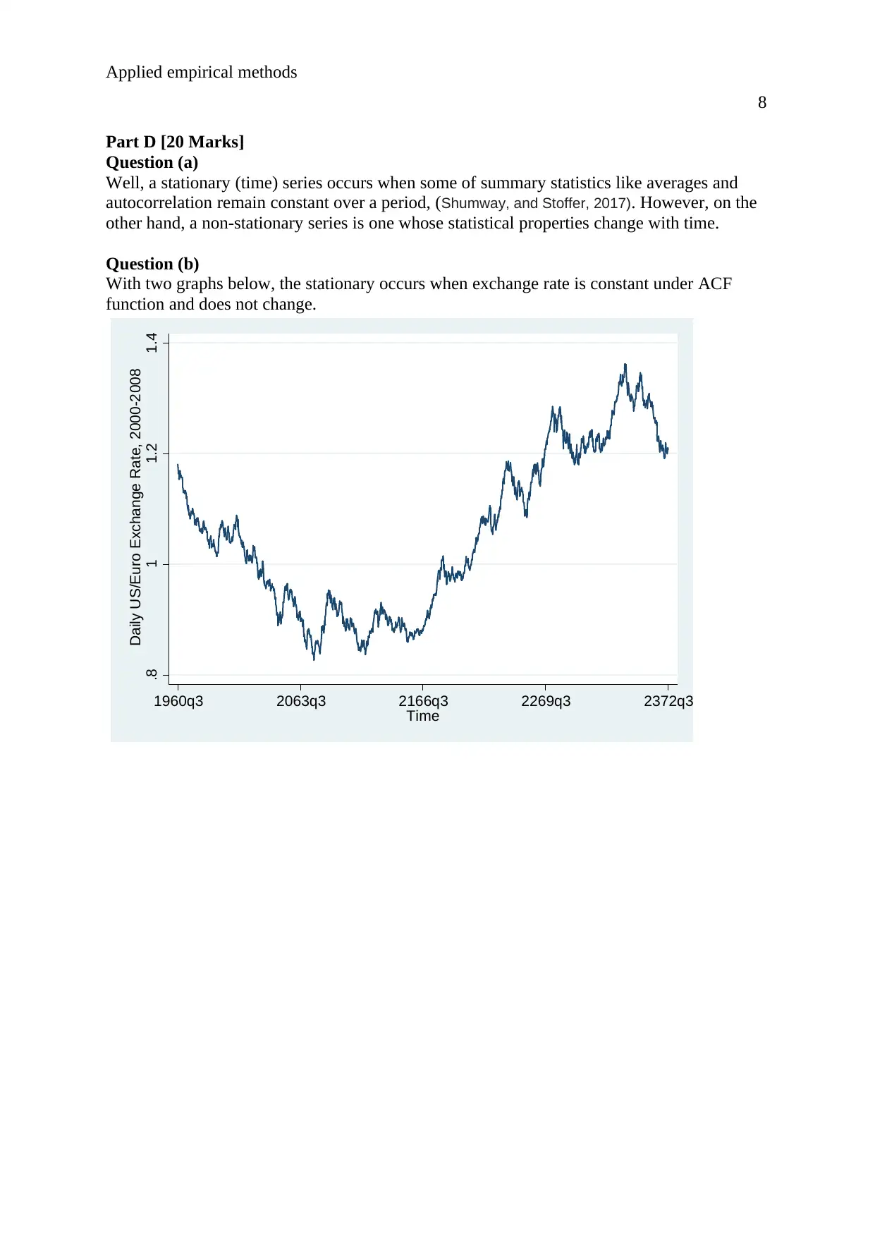
In both the models, the test scores are statistically significant with a slight reduction in the
coefficient values of the test scores.
_cons .2001607 .0202245 9.90 0.000 .1604802 .2398411
lscore .1073167 .0134543 7.98 0.000 .0809195 .133714
use_fin_aid .6560624 .0215773 30.41 0.000 .6137278 .698397
won_lottry Coef. Std. Err. t P>|t| [95% Conf. Interval]
Total 292.71392 1,170 .250182837 Root MSE = .35536
Adj R-squared = 0.4953
Residual 147.492294 1,168 .126277649 R-squared = 0.4961
Model 145.221625 2 72.6108127 Prob > F = 0.0000
F(2, 1168) = 575.01
Source SS df MS Number of obs = 1,171
(no endogenous regressors)
_cons -.0701221 .0037151 -18.88 0.000 -.0774111 -.0628332
won_lottry .0518653 .0064886 7.99 0.000 .0391347 .064596
use_fin_aid .6578609 .0065763 100.04 0.000 .6449583 .6707636
lscorez Coef. Std. Err. t P>|t| [95% Conf. Interval]
Total 145.253891 1,170 .124148625 Root MSE = .08092
Adj R-squared = 0.9473
Residual 7.64806351 1,168 .006548 R-squared = 0.9473
Model 137.605827 2 68.8029137 Prob > F = 0.0000
F(2, 1168) = 10507.47
Source SS df MS Number of obs = 1,171
Instrumental variables (2SLS) regression
Question 3
Basically, a good instrument should ensure that a predictor variable (x) in a regression model
is not correlated with the error term (e) in the model while dealing with endogeneity,
(Chesher, and Rosen, 2017). This is possible when several variables are standardized or
generating other variables by getting the product between the coefficient values and the
variable of interest, (Hayes, and Montoya, 2017).
_cons -.0701221 .0037151 -18.88 0.000 -.0774111 -.0628332
won_lottry .0518653 .0064886 7.99 0.000 .0391347 .064596
use_fin_aid .6578609 .0065763 100.04 0.000 .6449583 .6707636
lscorez Coef. Std. Err. t P>|t| [95% Conf. Interval]
Total 145.253891 1,170 .124148625 Root MSE = .08092
Adj R-squared = 0.9473
Residual 7.64806351 1,168 .006548 R-squared = 0.9473
Model 137.605827 2 68.8029137 Prob > F = 0.0000
F(2, 1168) = 10507.47
Source SS df MS Number of obs = 1,171
Question 4
From the endogeneity tests the IV results offers a more reliable estimate of the impact of the
intervention compared to the OLS.

Applied empirical methods
8
Part D [20 Marks]
Question (a)
Well, a stationary (time) series occurs when some of summary statistics like averages and
autocorrelation remain constant over a period, (Shumway, and Stoffer, 2017). However, on the
other hand, a non-stationary series is one whose statistical properties change with time.
Question (b)
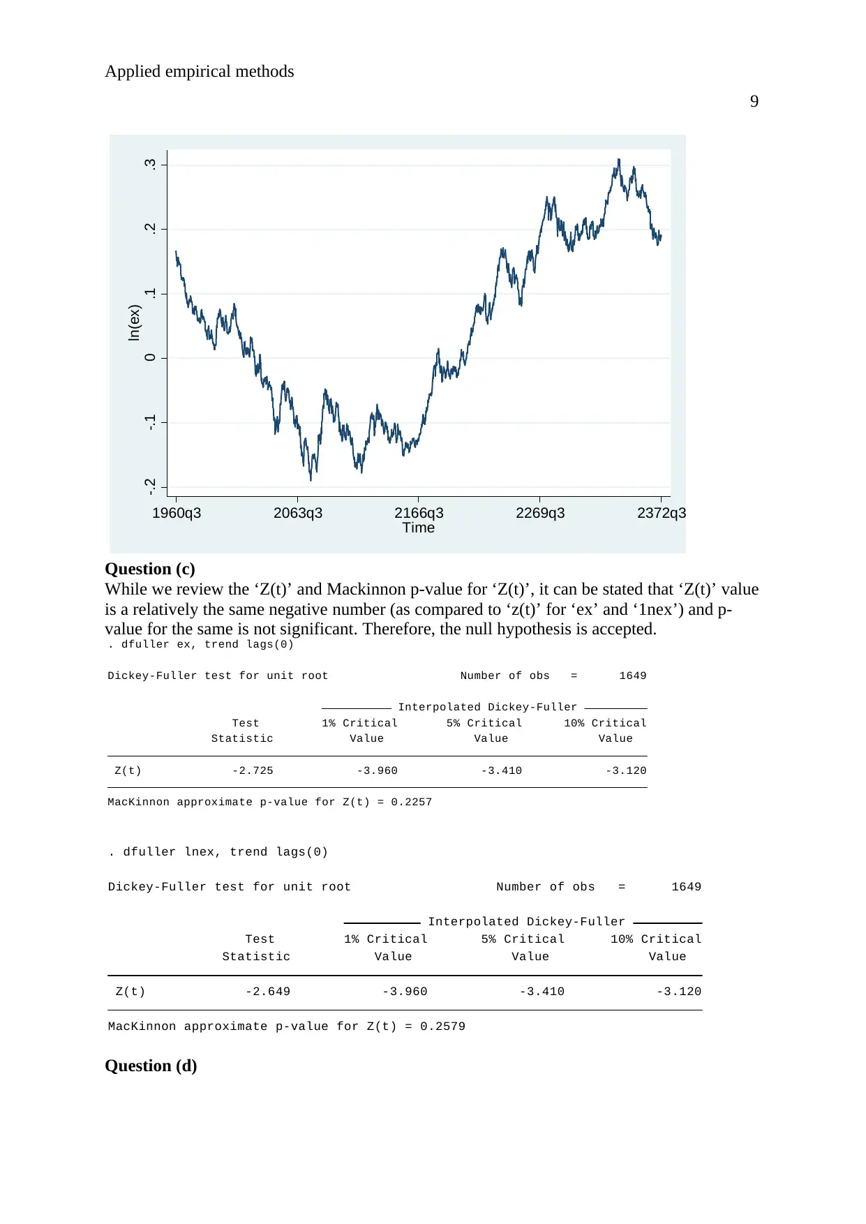
With two graphs below, the stationary occurs when exchange rate is constant under ACF
function and does not change.
.8 1 1.2 1.4
Daily US/Euro Exchange Rate, 2000-2008
1960q3 2063q3 2166q3 2269q3 2372q3
Time

Applied empirical methods
9
-.2 -.1 0 .1 .2 .3
ln(ex)
1960q3 2063q3 2166q3 2269q3 2372q3
Time
Question (c)
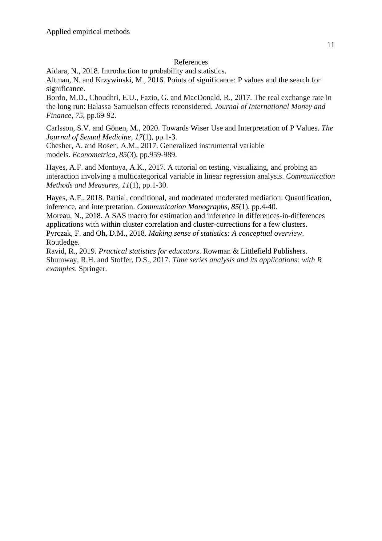
While we review the ‘Z(t)’ and Mackinnon p-value for ‘Z(t)’, it can be stated that ‘Z(t)’ value
is a relatively the same negative number (as compared to ‘z(t)’ for ‘ex’ and ‘1nex’) and p-
value for the same is not significant. Therefore, the null hypothesis is accepted.
MacKinnon approximate p-value for Z(t) = 0.2257
Z(t) -2.725 -3.960 -3.410 -3.120
Statistic Value Value Value
Test 1% Critical 5% Critical 10% Critical
Interpolated Dickey-Fuller
Dickey-Fuller test for unit root Number of obs = 1649
. dfuller ex, trend lags(0)
MacKinnon approximate p-value for Z(t) = 0.2579
Z(t) -2.649 -3.960 -3.410 -3.120
Statistic Value Value Value
Test 1% Critical 5% Critical 10% Critical
Interpolated Dickey-Fuller
Dickey-Fuller test for unit root Number of obs = 1649
. dfuller lnex, trend lags(0)
Question (d)

Applied empirical methods
10
Well, there is no change expected in the trend because the exchange rates seems to be
constant, (Bordo, Choudhri, Fazio, and MacDonald, 2017). For changes in conclusion to be seen
then timelines needs to be adjusted accordingly.

Applied empirical methods
11
References
Aidara, N., 2018. Introduction to probability and statistics.
Altman, N. and Krzywinski, M., 2016. Points of significance: P values and the search for
significance.
Bordo, M.D., Choudhri, E.U., Fazio, G. and MacDonald, R., 2017. The real exchange rate in
the long run: Balassa-Samuelson effects reconsidered. Journal of International Money and
Finance, 75, pp.69-92.
Carlsson, S.V. and Gönen, M., 2020. Towards Wiser Use and Interpretation of P Values. The
Journal of Sexual Medicine, 17(1), pp.1-3.
Chesher, A. and Rosen, A.M., 2017. Generalized instrumental variable
models. Econometrica, 85(3), pp.959-989.
Hayes, A.F. and Montoya, A.K., 2017. A tutorial on testing, visualizing, and probing an
interaction involving a multicategorical variable in linear regression analysis. Communication
Methods and Measures, 11(1), pp.1-30.
Hayes, A.F., 2018. Partial, conditional, and moderated moderated mediation: Quantification,
inference, and interpretation. Communication Monographs, 85(1), pp.4-40.
Moreau, N., 2018. A SAS macro for estimation and inference in differences-in-differences
applications with within cluster correlation and cluster-corrections for a few clusters.
Pyrczak, F. and Oh, D.M., 2018. Making sense of statistics: A conceptual overview.
Routledge.
Ravid, R., 2019. Practical statistics for educators. Rowman & Littlefield Publishers.
Shumway, R.H. and Stoffer, D.S., 2017. Time series analysis and its applications: with R
examples. Springer.

Applied empirical methods
12
Appendix
///////Do file prepared by the student///////////////////
/////Part A////////////////
//////////////Question (a)/////////
by treated , sort : summarize age test famwealth famsize
//////////////Question (b)/////////
ttest age, by(treated)
ttest test, by(treated)
ttest famwealth, by(treated)
ttest famsize, by(treated)
ttest sex, by(treated)
//////////////Question (c)/////////
ttest age, by(treated)
ttest test, by(treated)
ttest famwealth, by(treated)
ttest famsize, by(treated)
ttest sex, by(treated)
//////////////Question (d)/////////
regress treated age famwealth famsize test, robust
//////////////Question (d)/////////
//detecting outliers////
graph box test
graph box famwealth
graph box famsize
graph box age
/////generating new variables that are standadrdized/////
summarize age test famwealth famsize
gen z_age = (age-11.19398)/1.844226
gen z_test = (test-8.450665)/.5138679
gen z_famwealth = (famwealth-155576.4)/849719.9
gen z_famsize = (famsize-5.300266)/2.20517
regress treated z_age z_famwealth z_famsize z_test, robust
/////Part B////////////////
//////////////Question (a)/////////
ssc install diff
diff learnings , t(treated) p(t)
//////////////Question (b)/////////
diff learnings, treated(treated) period(t) cov(bk kfc mc wendy) kernel id(id)