QNM222 Statistics Assignment: Hypothesis Tests and Regression Model

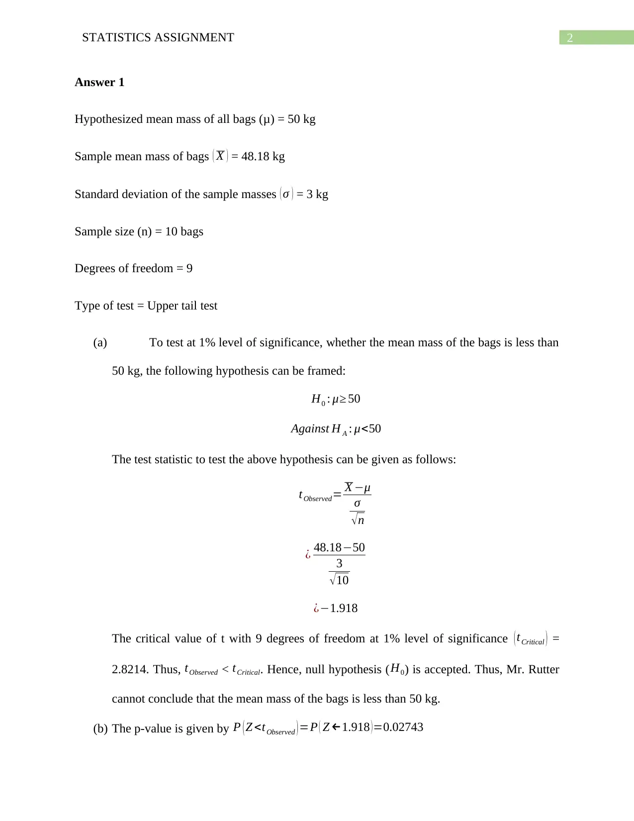
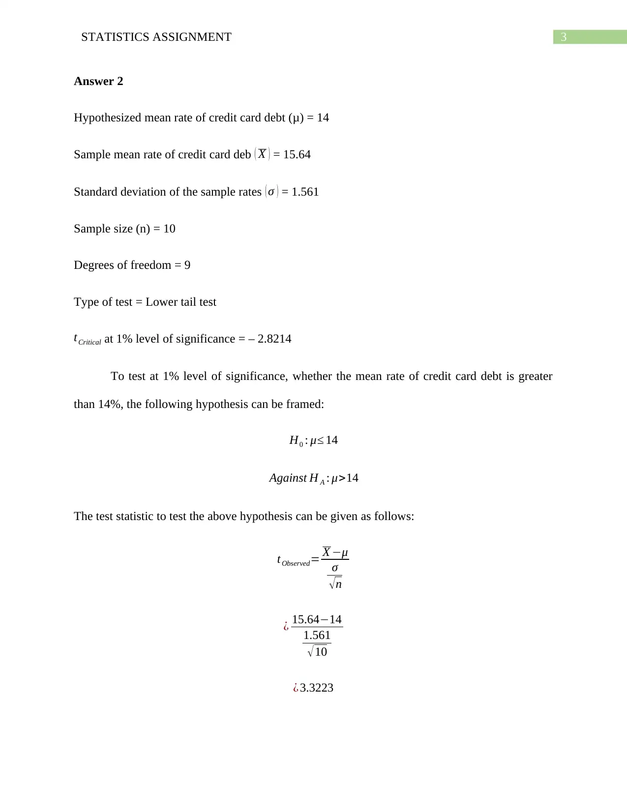
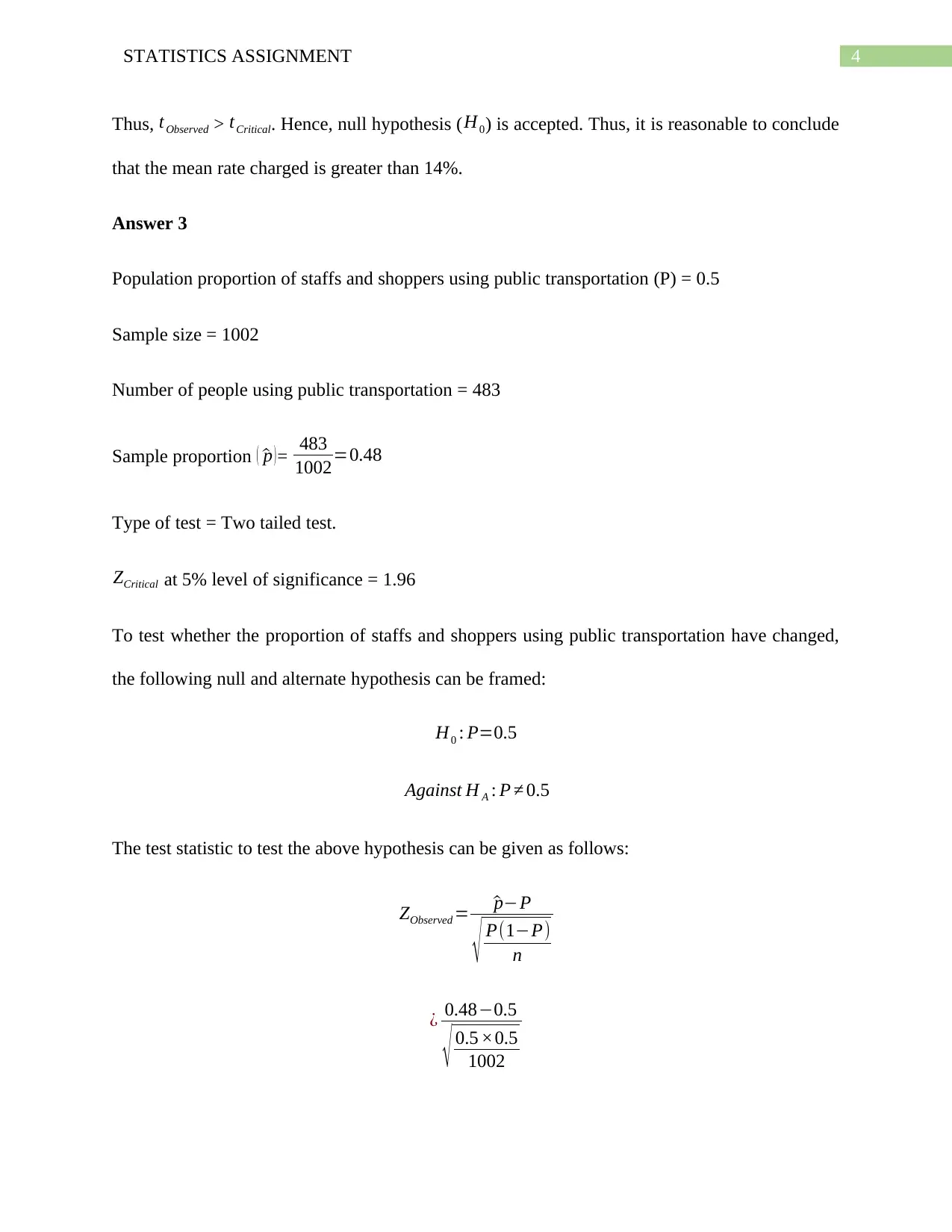
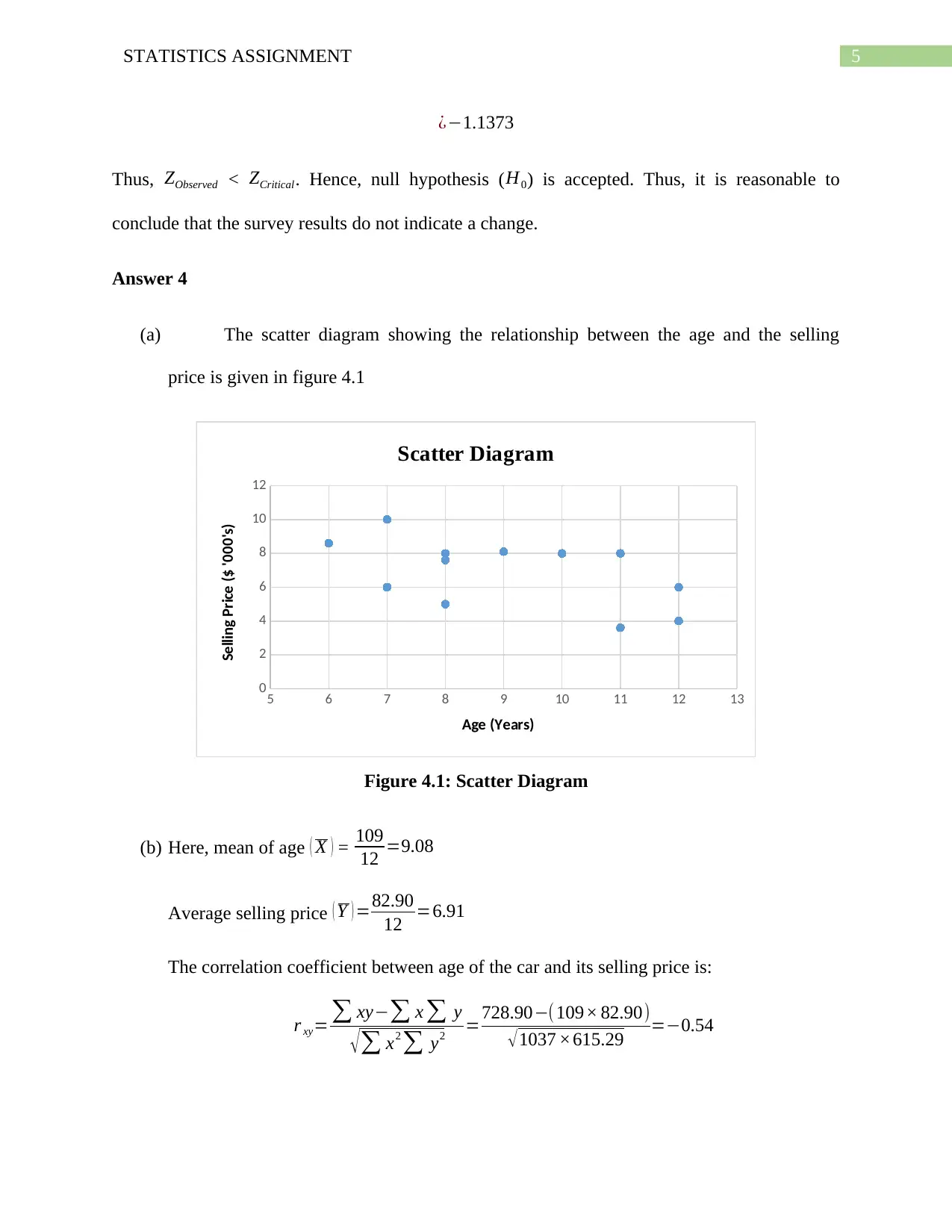
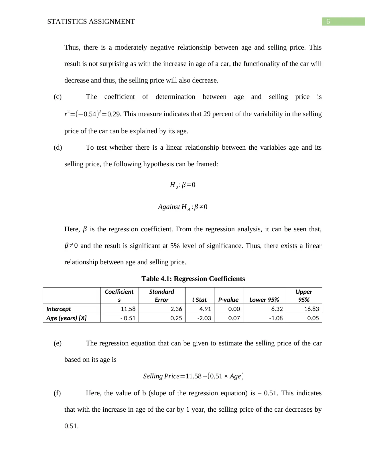
This statistics assignment solution addresses several problems related to hypothesis testing and regression analysis. The first question involves testing whether the mean mass of mulch bags is less than 50 kg using a t-test. The null hypothesis is accepted, indicating insufficient evidence to conclude the mean mass is less than 50 kg, and the p-value is calculated. The second question examines whether the mean rate of credit card debt is greater than 14%, again using a t-test, leading to the conclusion that the mean rate is reasonably greater than 14%. The third question tests whether the proportion of staff and shoppers using public transportation has changed, using a z-test, and concludes that the survey results do not indicate a change. Finally, the assignment includes a regression analysis to explore the relationship between the age of a car and its selling price, determining a moderately negative correlation and providing a regression equation to estimate the selling price based on age. The coefficient of determination indicates that 29% of the variability in selling price can be explained by age, and a hypothesis test confirms a linear relationship between the variables.

Running Head: STATISTICS ASSIGNMENT
Statistics Assignment
Name of the Student
Name of the University
Author Note

1STATISTICS ASSIGNMENT
Table of Contents
Answer 1..........................................................................................................................................2
Answer 2..........................................................................................................................................3
Answer 3..........................................................................................................................................4
Answer 4..........................................................................................................................................5

2STATISTICS ASSIGNMENT
Answer 1
Hypothesized mean mass of all bags (μ) = 50 kg
Sample mean mass of bags ( X ) = 48.18 kg
Standard deviation of the sample masses ( σ ) = 3 kg
Sample size (n) = 10 bags
Degrees of freedom = 9
Type of test = Upper tail test
(a) To test at 1% level of significance, whether the mean mass of the bags is less than
50 kg, the following hypothesis can be framed:
H0 : μ≥ 50
Against H A : μ<50
The test statistic to test the above hypothesis can be given as follows:
tObserved= X −μ
σ
√ n
¿ 48.18−50
3
√10
¿−1.918
The critical value of t with 9 degrees of freedom at 1% level of significance ( tCritical ) =
2.8214. Thus, tObserved < tCritical. Hence, null hypothesis ( H0) is accepted. Thus, Mr. Rutter
cannot conclude that the mean mass of the bags is less than 50 kg.
(b) The p-value is given by P ( Z <tObserved ) =P ( Z ←1.918 ) =0.02743

3STATISTICS ASSIGNMENT
Answer 2
Hypothesized mean rate of credit card debt (μ) = 14
Sample mean rate of credit card deb ( X ) = 15.64
Standard deviation of the sample rates ( σ ) = 1.561
Sample size (n) = 10
Degrees of freedom = 9
Type of test = Lower tail test
tCritical at 1% level of significance = – 2.8214
To test at 1% level of significance, whether the mean rate of credit card debt is greater
than 14%, the following hypothesis can be framed:
H0 : μ≤ 14
Against H A : μ>14
The test statistic to test the above hypothesis can be given as follows:
tObserved= X −μ
σ
√n
¿ 15.64−14
1.561
√ 10
¿ 3.3223

4STATISTICS ASSIGNMENT
Thus, tObserved > tCritical. Hence, null hypothesis (H0) is accepted. Thus, it is reasonable to conclude
that the mean rate charged is greater than 14%.
Answer 3
Population proportion of staffs and shoppers using public transportation (P) = 0.5
Sample size = 1002
Number of people using public transportation = 483
Sample proportion ( ^p )= 483
1002=0.48
Type of test = Two tailed test.
ZCritical at 5% level of significance = 1.96
To test whether the proportion of staffs and shoppers using public transportation have changed,
the following null and alternate hypothesis can be framed:
H0 : P=0.5
Against H A : P ≠ 0.5
The test statistic to test the above hypothesis can be given as follows:
ZObserved = ^p−P
√ P(1−P)
n
¿ 0.48−0.5
√ 0.5 ×0.5
1002

5STATISTICS ASSIGNMENT
¿−1.1373
Thus, ZObserved < ZCritical. Hence, null hypothesis (H0) is accepted. Thus, it is reasonable to
conclude that the survey results do not indicate a change.
Answer 4
(a) The scatter diagram showing the relationship between the age and the selling
price is given in figure 4.1
5 6 7 8 9 10 11 12 13
0
2
4
6
8
10
12
Scatter Diagram
Age (Years)
Selling Price ($ '000's)
Figure 4.1: Scatter Diagram
(b) Here, mean of age ( X ) = 109
12 =9.08
Average selling price ( Y ) =82.90
12 =6.91
The correlation coefficient between age of the car and its selling price is:
r xy= ∑ xy−∑ x ∑ y
√∑ x2
∑ y2 =728.90−(109× 82.90)
√1037 ×615.29 =−0.54

6STATISTICS ASSIGNMENT
Thus, there is a moderately negative relationship between age and selling price. This
result is not surprising as with the increase in age of a car, the functionality of the car will
decrease and thus, the selling price will also decrease.
(c) The coefficient of determination between age and selling price is
r2=(−0.54)2 =0.29. This measure indicates that 29 percent of the variability in the selling
price of the car can be explained by its age.
(d) To test whether there is a linear relationship between the variables age and its
selling price, the following hypothesis can be framed:
H0 : β=0
Against H A : β ≠0
Here, β is the regression coefficient. From the regression analysis, it can be seen that,
β ≠ 0 and the result is significant at 5% level of significance. Thus, there exists a linear
relationship between age and selling price.
Table 4.1: Regression Coefficients
Coefficient
s
Standard
Error t Stat P-value Lower 95%
Upper
95%
Intercept 11.58 2.36 4.91 0.00 6.32 16.83
Age (years) [X] - 0.51 0.25 -2.03 0.07 -1.08 0.05
(e) The regression equation that can be given to estimate the selling price of the car
based on its age is
Selling Price=11.58−(0.51 × Age)
(f) Here, the value of b (slope of the regression equation) is – 0.51. This indicates
that with the increase in age of the car by 1 year, the selling price of the car decreases by
0.51.

7STATISTICS ASSIGNMENT
(g) The estimated selling price of a 10-year-old car is:
Selling Price=11.58− ( 0.51× 10 )=6.44
Therefore, the required estimated selling price of a 10-year old car is $6,440