Optimization Assignment: Methods, Quadratic Functions, and Solutions

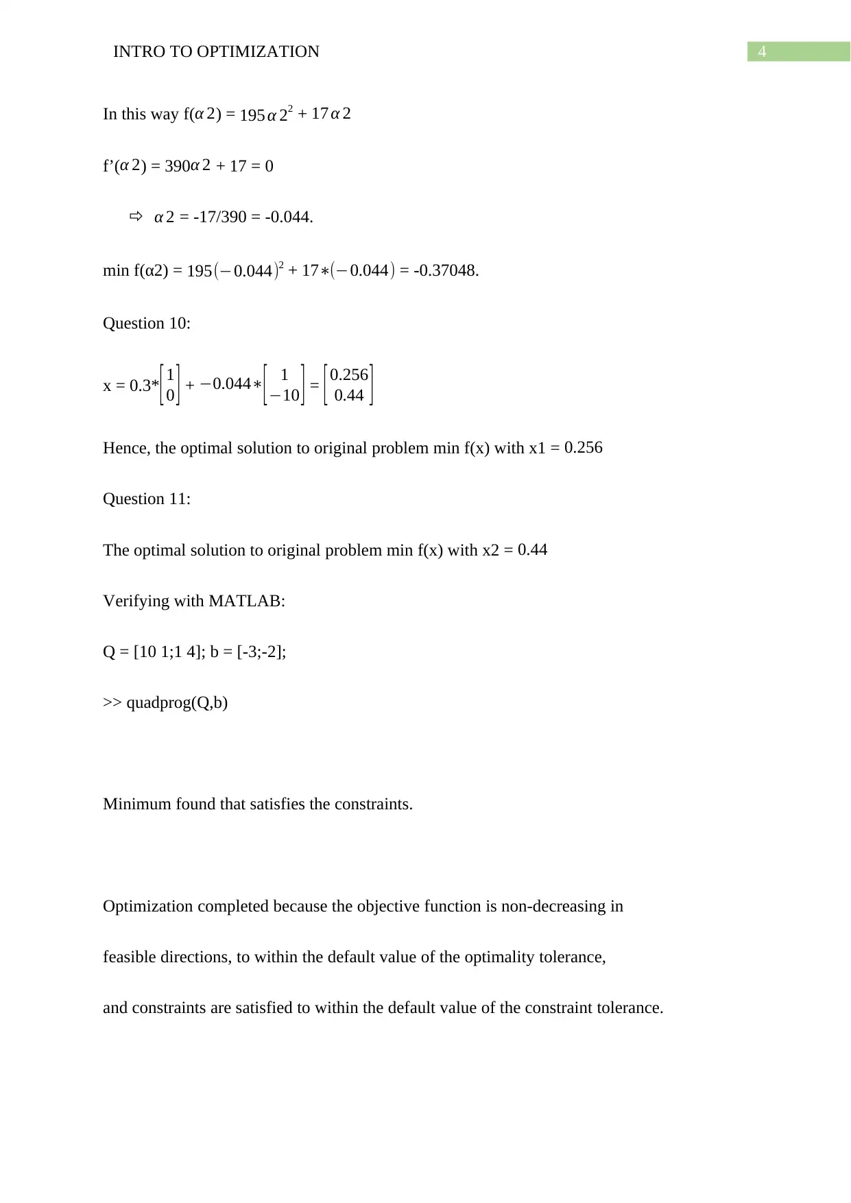
This assignment solution delves into optimization techniques, focusing on conjugate direction methods and their application to quadratic functions. The student addresses a series of questions, starting with a problem where the quadratic form's matrix is diagonal, allowing for separate optimization of variables. The solution progresses through the conjugate direction method, Gram-Schmidt process, and the Fletcher-Reeves conjugate gradient (FRCG) algorithm. It also explores constrained optimization using Lagrange multipliers and MATLAB code for verification. The assignment covers topics like finding optimal values, gradients, and the impact of constraint variations, providing a comprehensive understanding of optimization principles.

Running head: INTRO TO OPTIMIZATION
INTRO TO OPTIMIZATION
Name of the Student
Name of the University
Author Note

1INTRO TO OPTIMIZATION
Question 1:
Q = [10 0
0 4 ] b = [−3
−2 ]
Conjugate direction method finds basis where the components of x minimizes
f(x) = (½)x^T*Q*x + b^T*x
= (½)*[x1 x2]* [ 10 0
0 4 ]*[ x 1
x 2 ] + [−3 −2 ]*[ x 1
x 2 ]
= [x1/2 x2/2] [10 x 1
4 x 2 ] -3x1 -2x2
= 5 x 12 +2 x 22 – 3 x 1 – 2 x 2
Hence, 1? = 5, 2? = 2, 3? = 3 and 4? = 2
Question 2:
f(x) = f(x1) + f(x2)
f(x1) = 5 x 12−3 x 1
f(x2) = 2 x 22−2 x 2
Now, f(x1) is minimum when f’(x1) = 0
 10x1 – 3 = 0
 x1 = 3/10
f’’(x1) = 10, f’’(3/10) = 10 > 0 (Hence, there is minimum of f(x1) at x1 = 3/10.
Thus optimal solution to min(f(x1)) is at x1 = 3/10 with f(3/10) = 5*(3/10)^2 – 3*(3/10)
= -0.45.

2INTRO TO OPTIMIZATION
Question 3:
Similarly, min(f(x2)) is found by
f’(x2) = 0
 4x2 – 2 = 0
 x2 = 2/4 = ½.
Then the optimal solution of f(x2) = 2∗0.52−2∗0.5 = -0.5 at x2 = ½.
Question 4:
Hence, the optimal value f(x1,x2) = 5∗( 0.3 )2 +2∗0.52 – 3∗0.3 – 2∗0.5 = -0.95.
At x1= 0.3
Question 5:
Min f(x1,x2) = -0.95
At x2 = 0.5.
Question 6:
Given, Q = [10 1
1 4 ] and d1 = [ 1
0 ] and first element of d2 is 1.
Let, d2 = [ 1
d ]
Hence, d 1T∗Q∗d 2=0
 [1¿ 0]∗
[ 10 1
1 4 ]∗
[ 1
d ] = 0
 [1¿ 0] [ 10+d
1+4 d ] = 0

3INTRO TO OPTIMIZATION
 10+d = 0
 d=−10
Hence, the second element of d2 = -10.
Question 7:
Now, x = α1*d1 + α2*d2
= α 1 [1
0 ] + α2[ 1
−10 ] = [α 1+α 2
−10 α 2 ]
Hence, f(α1,α2) = (½)*[ α 1+α 2 −10 α 2 ]*[ 10 1
1 4 ]∗
[ α 1+ α 2
−10 α 2 ] + [ −3 −2 ] [ α 1+α 2
−10 α 2 ]
= (1/2) [ α 1+ α 2 −10 α 2 ] [ 10 α 1
α 1−39 α 2 ] + −3 α 1+17 α 2
= (½)(10 α 12 +10 α 1 α 2−10 α 1 α 2+390 α 22 ) −3 α 1+17 α 2
= 5 α 12 +195 α 22−3 α 1+ 17 α 2
Hence, 1? = 5, 2? = 195, 3? = -3 and 4? = 17
Question 8:
f(α1,α2) = f(α1) + f(α 2)
f(α1) = 5 α 12−3 α 1
f’(α1) = 10 α 1 – 3
f’(α1) = 0 => α 1 = 3/10
Hence, min f(α1) = 5∗0.32−3∗0.3 = -0.45.
Question 9:

4INTRO TO OPTIMIZATION
In this way f(α 2) = 195 α 22 + 17 α 2
f’(α 2) = 390 α 2 + 17 = 0
 α 2 = -17/390 = -0.044.
min f(α2) = 195(−0.044)2 + 17∗(−0.044) = -0.37048.
Question 10:
x = 0.3* [ 1
0 ] + −0.044∗
[ 1
−10 ] = [ 0.256
0.44 ]
Hence, the optimal solution to original problem min f(x) with x1 = 0.256
Question 11:
The optimal solution to original problem min f(x) with x2 = 0.44
Verifying with MATLAB:
Q = [10 1;1 4]; b = [-3;-2];
>> quadprog(Q,b)
Minimum found that satisfies the constraints.
Optimization completed because the objective function is non-decreasing in
feasible directions, to within the default value of the optimality tolerance,
and constraints are satisfied to within the default value of the constraint tolerance.

5INTRO TO OPTIMIZATION
<stopping criteria details>
ans =
0.2564
0.4359
Thus it can be seen that the theoretically found values of x components is approximately
equal to quadprog() function output.
Question 12:
Q = [10 1
1 4 ]
Given Gram-Schmidt process y1 = u = [ 1
0 ]and y2 = v = [ 0
1 ]
d1 and d2 are taken from same subspace of linear independent vectors.
Hence, d1 = [ 1
0 ] and d2 = [0
1 ]
Thus by Gram-Schmidt process
[ ( d 2 )1
( d 2 )2 ] = -[ 0
1 ] + ¿*[ 10 1
1 4 ]*[ 1
0 ] ¿/¿*[ 10 1
1 4 ]*[ 1
0 ] ¿ ¿∗
[ 1
0 ] +
¿*[ 10 1
1 4 ]*[ 0
1 ] ¿/¿*[ 10 1
1 4 ]*[ 0
1 ] ¿ ¿∗
[ 0
1 ]
= - [0
1 ] + [0.1
0 ] + [0
1 ]

6INTRO TO OPTIMIZATION
= [0.1
0 ]
Hence, ( d 2 )1 = 0.1
Question 13:
By Gram-Schmidt process ( d 2 ) 2 = 0
Question 14:
f(x) = (½)x^T*Q*x + b^T*x
∇ f (x ) = (d/dx)(Qx^2/2 + b^T*x) = Qx + b^T
Hence, 1? = Q
Question 15:
And 2? = b^T
Question 16:
Given, the minimization problem
min f(x1,x2) = 1000/(x1 + x2) + (x1 – 4)^2 + (x2-10)^2
The FRCG algorithm is given by,
dk +1 = -∇ f ( xk+1 ) + ||∇ f ( xk +1 )||2
||∇ f ( xk )||2 dk
x^0 = [3
1 ]
x1 = -[3
1 ] + [ 1 1
−4 −10 ]∗[1
0 ] = -[ 3
1 ] + [ 1
−4 ] = [−2
−5 ]

7INTRO TO OPTIMIZATION
Hence, x1
(1) = -2
Question 17:
As found from above x2
(1) = -5
Question 18:
Now, in the next iteration
x2 = -[−2
−5 ] + [ 1 1
−4 −10 ]∗[ 1
0 ] = -[−2
−5 ]+ [ 1
−4 ]= [3
1 ]
Hence, x1
(2) = 3
Question 19:
From the previous calculation
x2
(2) = 1
Question 20:
Given, problem
max f(x1,x2) = x 1∗x 22
s.t
2 x 12 +3 x 22=1
 x 22 =1 – 2 x 12
3
Putting expression of x 22 in objective function gives
max f(x1) = x1* 1 – 2 x 12
3 = x 1
3 − 2
3 x 13

8INTRO TO OPTIMIZATION
Hence, f’(x1) = 1/3 – 2x1^2 = 0
 x1 = ±sqrt(1/6)
Now, f’’(x1) = -4x1
f’’(sqrt(1/6)) < 0 (hence there is a maximum)
f’’(-sqrt(1/6)) > 0 (hence there is a minimum)
Thus at x1 = sqrt(1/6) = 0.4082 there exists a maximum.
Question 21:
Now, when x1 = 0.4082
2*0.4082^2 + 3x2^2 = 1
 3x2^2 = 0.667
 x2 = ±0.4714
Question 22:
MATLAB code:
e1= ezplot('2*x^2+9*y^2=1'); axis equal; hold on
e2 = ezplot('x*y^2=0.1'); hold on;
e3 = ezplot('x*y^2=0.3'); hold on;
e4 = ezplot('x*y^2=0.5');
set(e1,'color',[1 0 0]);
set(e2,'color',[1 1 0]);
set(e3,'color',[0 1 1]);
set(e4,'color',[0 0 1])
grid on;
legend('2x^2+9y^2=1','xy^2=0.1','xy^2=0.3','xy^2=0.5','location','best')
title('Contour plots')
Plot:

9INTRO TO OPTIMIZATION
Contour plots
-6 -4 -2 0 2 4 6
x
-6
-4
-2
0
2
4
6
y
2x2+9y2=1
xy2=0.1
xy2=0.3
xy2=0.5
Question 23:
[ y2
2 xy ] =λ [ 4 x
6 y ]
Or, y^2 = 4 xλ (1)
2 xy=6 yλ (2)
2x^2 + 3y^2 – 1= 0 (3)
From (2) 2x = 6λ => λ = x/3 (As y≠0 as seen from above plot)
2x^2 + 12 x∗x
3 – 1 = 0
2x^2 + 4x^2 = 1
 x^2 = 1/6 => x = ±sqrt(1/6)

10INTRO TO OPTIMIZATION
From the plot it can be seen all x values of xy^2 exists for x>0
Hence, x = -sqrt(1/6) is rejected.
Thus the optimal f(x,y) is for x = sqrt(1/6).
Thus λ = sqrt(1/6)/3 = 0.136.
Question 24:
From previous calculation x = 0.408.
Question 25:
y^2 = 4*0.408*0.136 => y = ±0.471
Question 26:
The optimal value of the objective function is f(0.408, ±0.471) = 0.408*(±0.471)^2 = 0.0905.
Question 27:
L(x,y,λ) = f(x,y) – λh(x,y)
∂ L
∂ x = ∂ f
∂ x −λ ∂ h
∂ x
Hence, 1? = λ
Question 28:
From previous calculation
∂ L
∂ y = ∂ f
∂ y −λ ∂ h
∂ y
2? = λ
Question 29:

11INTRO TO OPTIMIZATION
From question 27
∂ L
∂ y =−h(x , y )
3? = −h( x , y)
Question 30:
Given constraint of the problem is 2x^2 + 3y^2 = 1.01
Hence, a= 1.01 – 1 = 0.01.
Thus by using property the value of the objective function will increase by a factor λa.
λa = 0.136*0.01 = 0.00136.
Thus approximately the optimal value of the objective function f(x,y) = xy^2 will be
0.0905 + 0.00136 = 0.09186.
Question 31:
[ y2
2 xy ]=λ [4 x
6 y ]
Or, y^2 = 4 xλ (1)
2 xy=6 yλ (2)
2x^2 + 3y^2 – 1.01= 0 (3)
=> λ = x/3
2x^2 + 12 x∗x
3 – 1.01 = 0
 2x^2 + 4x^2 = 1.01
 x^2 = 1.01/6 = 0.168