Quantitative Analysis for Development Practice: Homework Solution

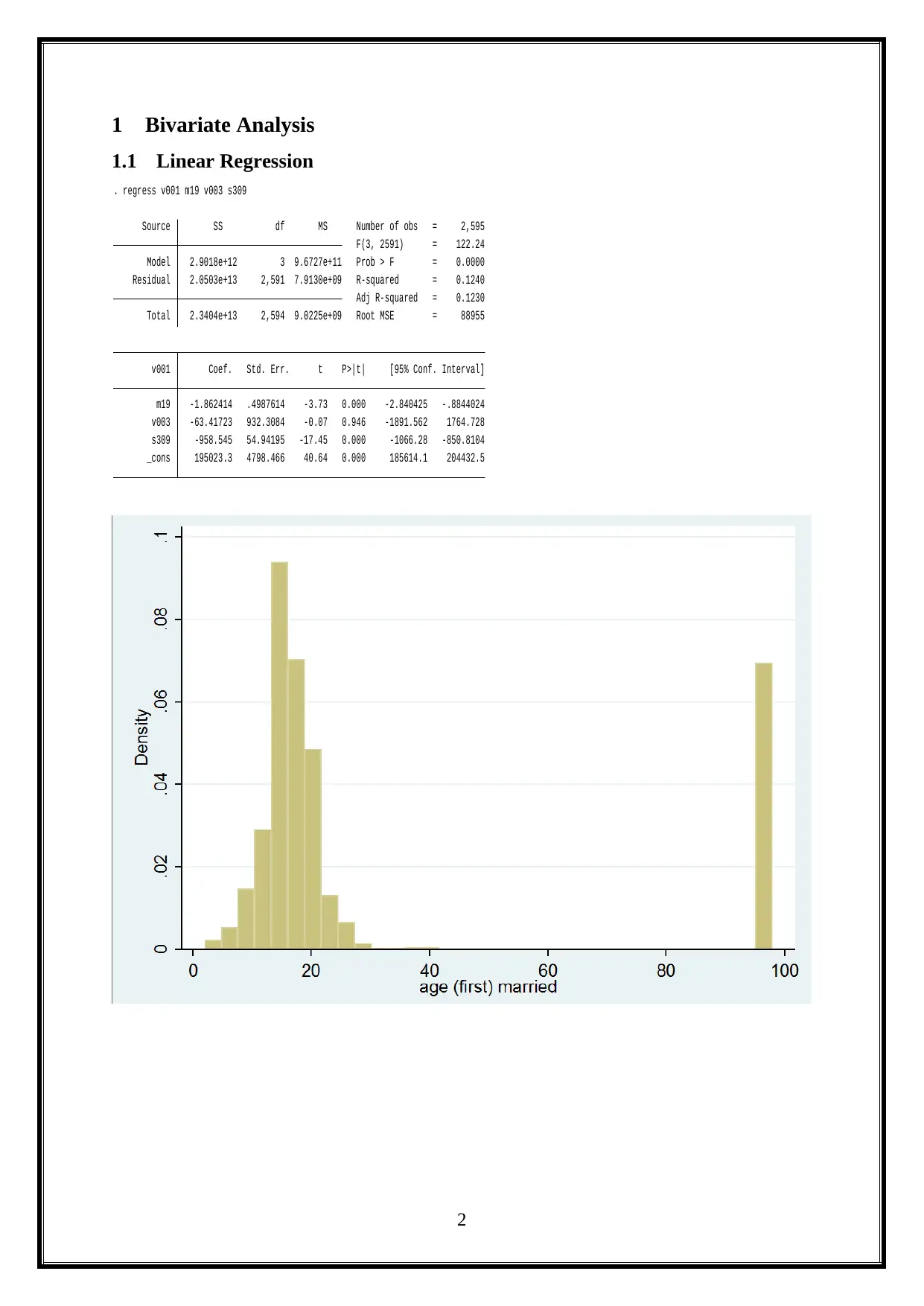
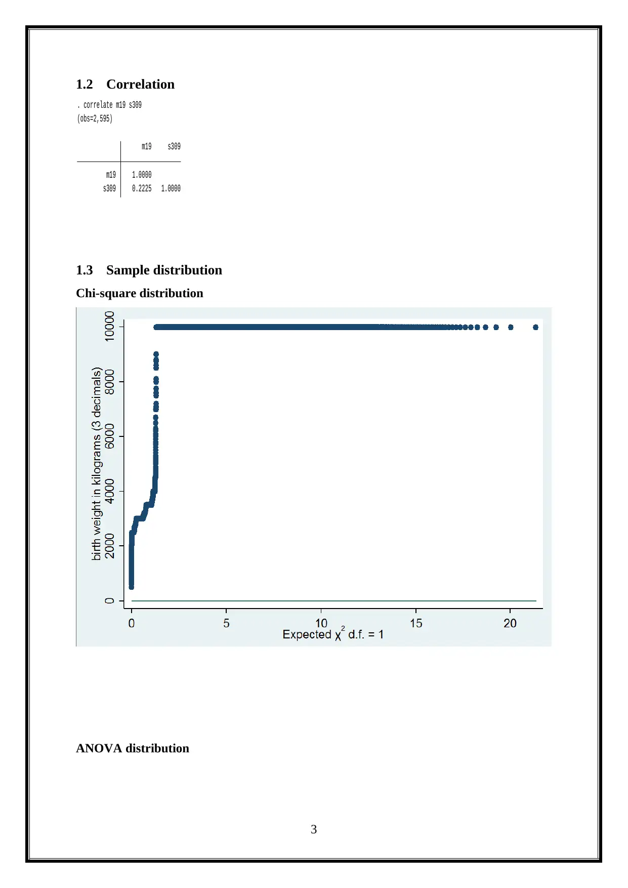
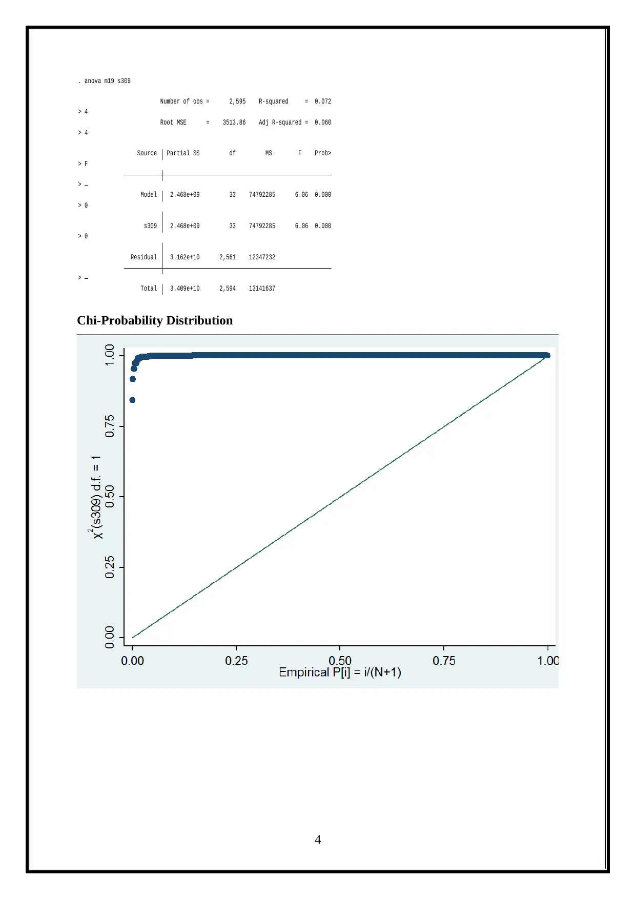
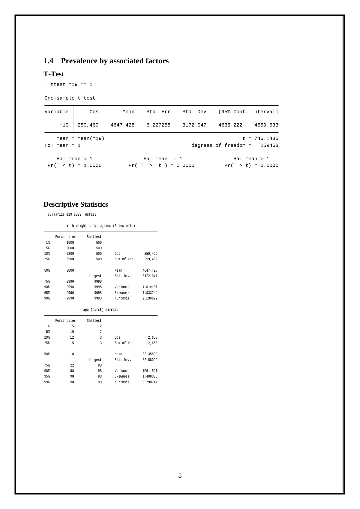
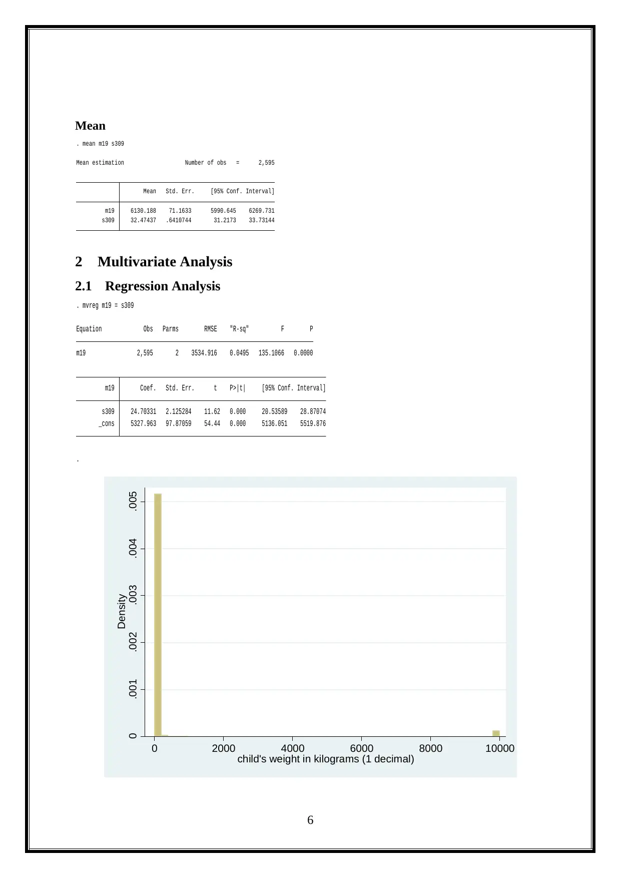
This assignment solution focuses on quantitative analysis for development practice, presenting a comprehensive analysis of statistical methods. It begins with bivariate analysis, exploring linear regression, correlation, sample distribution, and prevalence by associated factors. The solution then progresses to multivariate analysis, specifically regression analysis, providing detailed outputs and interpretations. The document includes statistical outputs, such as regression tables, correlation matrices, and descriptive statistics, to illustrate the concepts. Furthermore, the assignment analyzes sample distribution using ANOVA and Chi-square tests, and also provides prevalence analysis using t-tests and descriptive statistics to show the relationship between variables. The solution also includes Cronbach's alpha to measure the reliability of the scale. This assignment is a valuable resource for students studying quantitative methods in development practice, offering practical examples and explanations of statistical techniques.

Quantitative Analysis for Development Practice

Table of Contents
1 Bivariate Analysis.............................................................................................................2
1.1 Linear Regression......................................................................................................2
1.2 Correlation.................................................................................................................3
1.3 Sample distribution...................................................................................................3
1.4 Prevalence by associated factors..............................................................................5
2 Multivariate Analysis.......................................................................................................6
2.1 Regression Analysis...................................................................................................6
1

1 Bivariate Analysis
1.1 Linear Regression
_cons 195023.3 4798.466 40.64 0.000 185614.1 204432.5
s309 -958.545 54.94195 -17.45 0.000 -1066.28 -850.8104
v003 -63.41723 932.3084 -0.07 0.946 -1891.562 1764.728
m19 -1.862414 .4987614 -3.73 0.000 -2.840425 -.8844024
v001 Coef. Std. Err. t P>|t| [95% Conf. Interval]
Total 2.3404e+13 2,594 9.0225e+09 Root MSE = 88955
Adj R-squared = 0.1230
Residual 2.0503e+13 2,591 7.9130e+09 R-squared = 0.1240
Model 2.9018e+12 3 9.6727e+11 Prob > F = 0.0000
F(3, 2591) = 122.24
Source SS df MS Number of obs = 2,595
. regress v001 m19 v003 s309
2

1.2 Correlation
s309 0.2225 1.0000
m19 1.0000
m19 s309
(obs=2,595)
. correlate m19 s309
1.3 Sample distribution
Chi-square distribution
ANOVA distribution
3

Total 3.409e+10 2,594 13141637
>
Residual 3.162e+10 2,561 12347232
> 0
s309 2.468e+09 33 74792285 6.06 0.000
> 0
Model 2.468e+09 33 74792285 6.06 0.000
>
> F
Source Partial SS df MS F Prob>
> 4
Root MSE = 3513.86 Adj R-squared = 0.060
> 4
Number of obs = 2,595 R-squared = 0.072
. anova m19 s309
Chi-Probability Distribution
4

1.4 Prevalence by associated factors
T-Test
.
Pr(T < t) = 1.0000 Pr(|T| > |t|) = 0.0000 Pr(T > t) = 0.0000
Ha: mean < 1 Ha: mean != 1 Ha: mean > 1
Ho: mean = 1 degrees of freedom = 259468
mean = mean(m19) t = 746.1435
m19 259,469 4647.428 6.227258 3172.047 4635.222 4659.633
Variable Obs Mean Std. Err. Std. Dev. [95% Conf. Interval]
One-sample t test
. ttest m19 == 1
Descriptive Statistics
99% 98 98 Kurtosis 3.290744
95% 98 98 Skewness 1.488036
90% 98 98 Variance 1061.521
75% 22 98
Largest Std. Dev. 32.58099
50% 18 Mean 32.35892
25% 15 3 Sum of Wgt. 2,658
10% 12 3 Obs 2,658
5% 10 2
1% 5 2
Percentiles Smallest
age (first) married
99% 9998 9998 Kurtosis 2.199629
95% 9996 9998 Skewness 1.033744
90% 9996 9998 Variance 1.01e+07
75% 9996 9998
Largest Std. Dev. 3172.047
50% 3000 Mean 4647.428
25% 2500 500 Sum of Wgt. 259,469
10% 2200 500 Obs 259,469
5% 2000 500
1% 1500 500
Percentiles Smallest
birth weight in kilograms (3 decimals)
. summarize m19 s309, detail
5

Mean
s309 32.47437 .6410744 31.2173 33.73144
m19 6130.188 71.1633 5990.645 6269.731
Mean Std. Err. [95% Conf. Interval]
Mean estimation Number of obs = 2,595
. mean m19 s309
2 Multivariate Analysis
2.1 Regression Analysis
.
_cons 5327.963 97.87059 54.44 0.000 5136.051 5519.876
s309 24.70331 2.125284 11.62 0.000 20.53589 28.87074
m19 Coef. Std. Err. t P>|t| [95% Conf. Interval]
m19 2,595 2 3534.916 0.0495 135.1066 0.0000
Equation Obs Parms RMSE "R-sq" F P
. mvreg m19 = s3090 .001 .002 .003 .004 .005
Density
0 2000 4000 6000 8000 10000
child's weight in kilograms (1 decimal)
6

Cronbach’s alpha
.
Scale reliability coefficient: 0.0053
Number of items in the scale: 2
Average interitem covariance: 26345.69
Test scale = mean(unstandardized items)
. alpha m19 s309
7