Quantitative Analysis of Business Project: Analysis & Findings

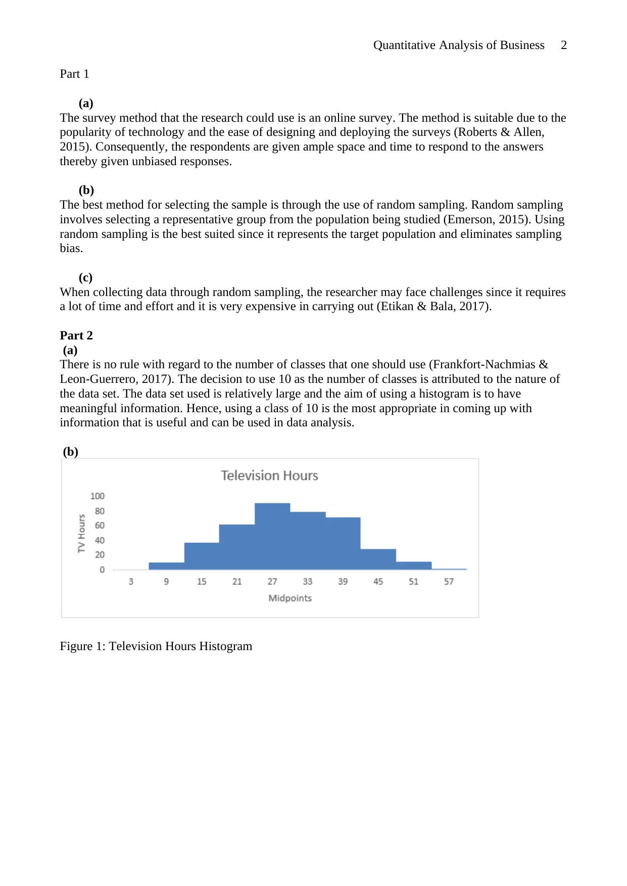
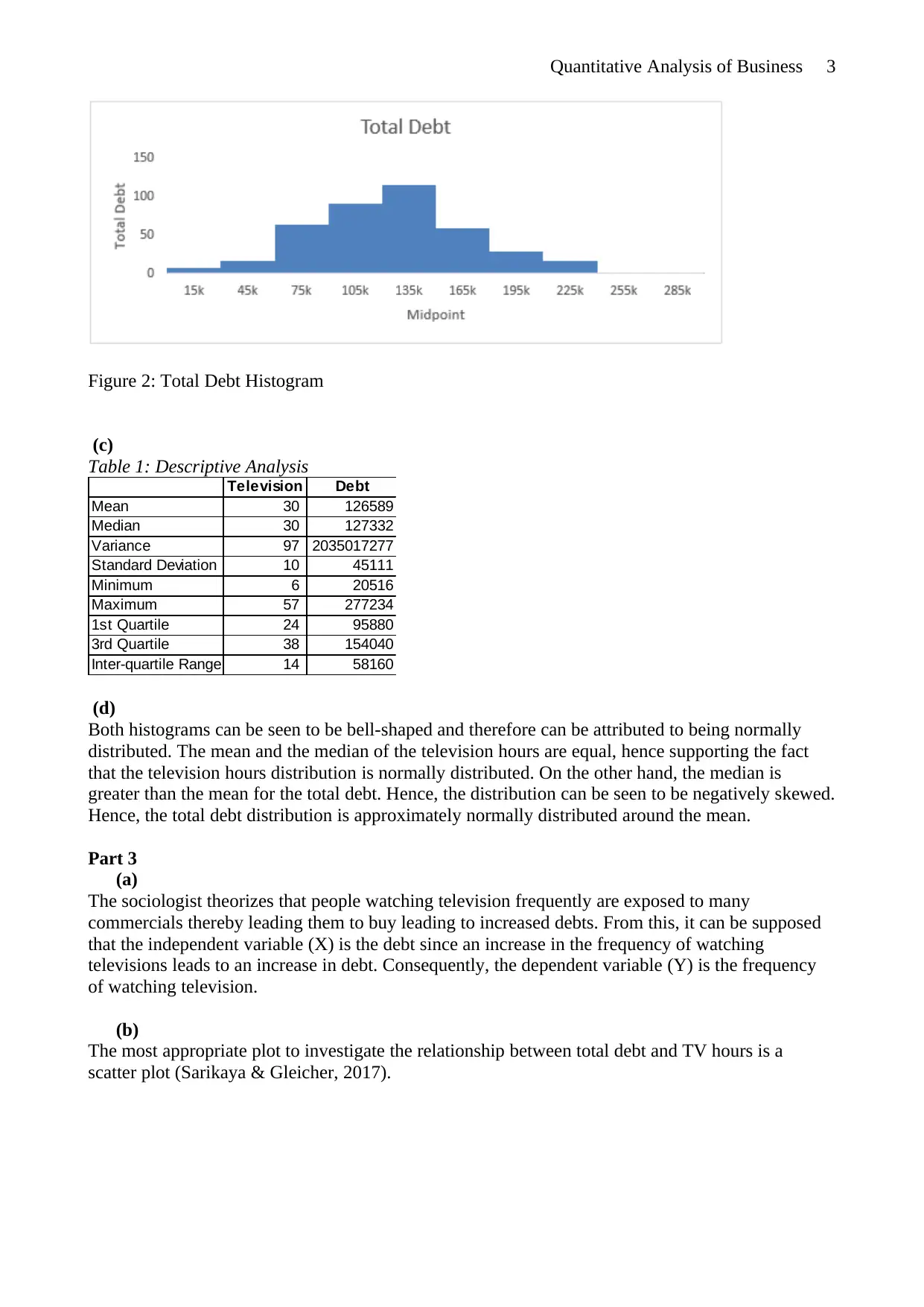
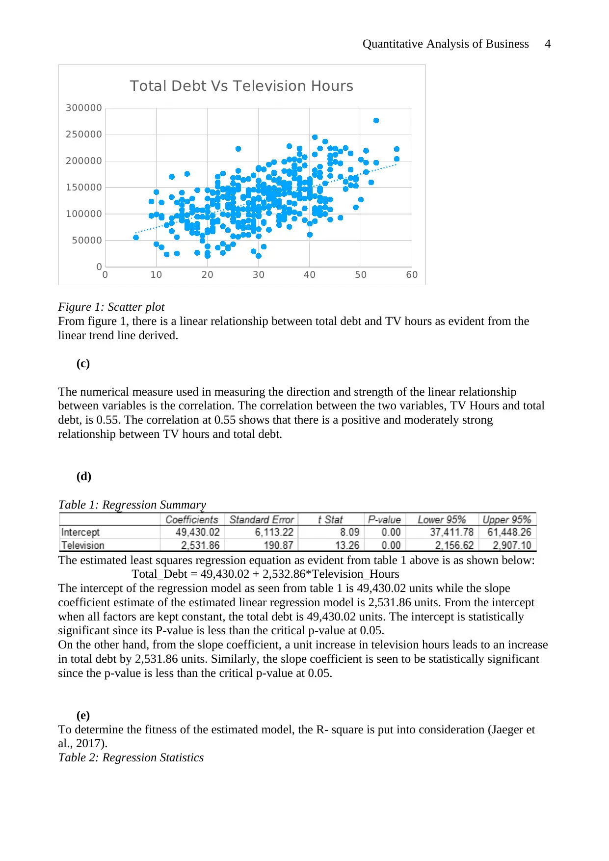
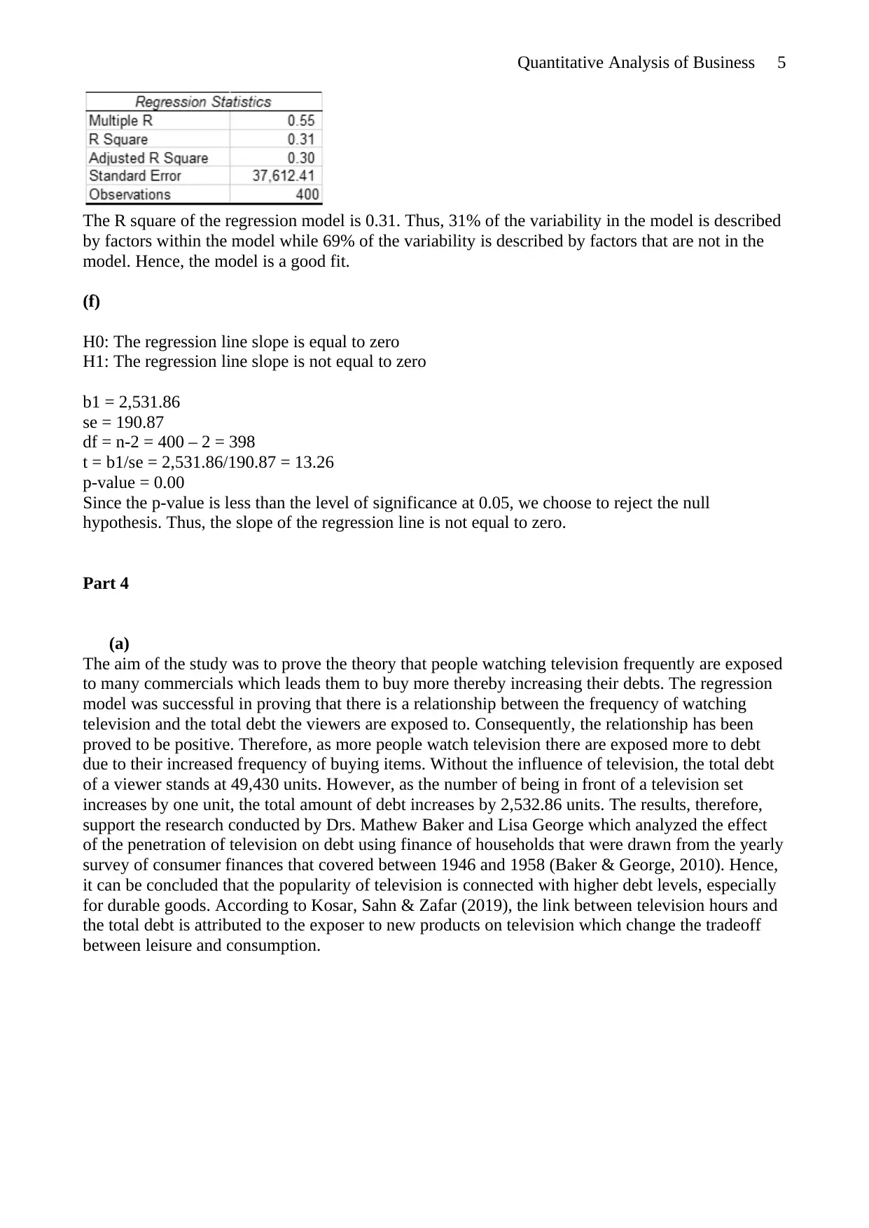
This assignment is a comprehensive quantitative analysis project focused on business applications. The project utilizes an online survey method to collect data, followed by a random sampling technique to ensure a representative sample. The analysis involves creating histograms to visualize data distributions, with a class size of 10 deemed appropriate for the dataset's size. Descriptive statistics, including mean and median, are calculated to understand the data's characteristics. A scatter plot is used to investigate the relationship between television viewing hours and total debt, revealing a positive correlation. Regression analysis is performed to quantify this relationship, resulting in a regression equation and statistical significance tests. The findings support the theory that increased television viewing is linked to higher debt levels due to exposure to commercials, aligning with existing research on the topic. The project concludes by interpreting the results and discussing the implications for consumer behavior and debt accumulation.

Running Header: Quantitative Analysis of Business 1
Quantitative Analysis for Business
Student’s name:
Student’s ID:
Institution:

Quantitative Analysis of Business 2
Part 1
(a)
The survey method that the research could use is an online survey. The method is suitable due to the
popularity of technology and the ease of designing and deploying the surveys (Roberts & Allen,
2015). Consequently, the respondents are given ample space and time to respond to the answers
thereby given unbiased responses.
(b)
The best method for selecting the sample is through the use of random sampling. Random sampling
involves selecting a representative group from the population being studied (Emerson, 2015). Using
random sampling is the best suited since it represents the target population and eliminates sampling
bias.
(c)
When collecting data through random sampling, the researcher may face challenges since it requires
a lot of time and effort and it is very expensive in carrying out (Etikan & Bala, 2017).
Part 2
(a)
There is no rule with regard to the number of classes that one should use (Frankfort-Nachmias &
Leon-Guerrero, 2017). The decision to use 10 as the number of classes is attributed to the nature of
the data set. The data set used is relatively large and the aim of using a histogram is to have
meaningful information. Hence, using a class of 10 is the most appropriate in coming up with
information that is useful and can be used in data analysis.
(b)
Figure 1: Television Hours Histogram

Quantitative Analysis of Business 3
Figure 2: Total Debt Histogram
(c)
Table 1: Descriptive Analysis
Television Debt
Mean 30 126589
Median 30 127332
Variance 97 2035017277
Standard Deviation 10 45111
Minimum 6 20516
Maximum 57 277234
1st Quartile 24 95880
3rd Quartile 38 154040
Inter-quartile Range 14 58160
(d)
Both histograms can be seen to be bell-shaped and therefore can be attributed to being normally
distributed. The mean and the median of the television hours are equal, hence supporting the fact
that the television hours distribution is normally distributed. On the other hand, the median is
greater than the mean for the total debt. Hence, the distribution can be seen to be negatively skewed.
Hence, the total debt distribution is approximately normally distributed around the mean.
Part 3
(a)
The sociologist theorizes that people watching television frequently are exposed to many
commercials thereby leading them to buy leading to increased debts. From this, it can be supposed
that the independent variable (X) is the debt since an increase in the frequency of watching
televisions leads to an increase in debt. Consequently, the dependent variable (Y) is the frequency
of watching television.
(b)
The most appropriate plot to investigate the relationship between total debt and TV hours is a
scatter plot (Sarikaya & Gleicher, 2017).

Quantitative Analysis of Business 4
0 10 20 30 40 50 60
0
50000
100000
150000
200000
250000
300000
Total Debt Vs Television Hours
Figure 1: Scatter plot
From figure 1, there is a linear relationship between total debt and TV hours as evident from the
linear trend line derived.
(c)
The numerical measure used in measuring the direction and strength of the linear relationship
between variables is the correlation. The correlation between the two variables, TV Hours and total
debt, is 0.55. The correlation at 0.55 shows that there is a positive and moderately strong
relationship between TV hours and total debt.
(d)
Table 1: Regression Summary
The estimated least squares regression equation as evident from table 1 above is as shown below:
Total_Debt = 49,430.02 + 2,532.86*Television_Hours
The intercept of the regression model as seen from table 1 is 49,430.02 units while the slope
coefficient estimate of the estimated linear regression model is 2,531.86 units. From the intercept
when all factors are kept constant, the total debt is 49,430.02 units. The intercept is statistically
significant since its P-value is less than the critical p-value at 0.05.
On the other hand, from the slope coefficient, a unit increase in television hours leads to an increase
in total debt by 2,531.86 units. Similarly, the slope coefficient is seen to be statistically significant
since the p-value is less than the critical p-value at 0.05.
(e)
To determine the fitness of the estimated model, the R- square is put into consideration (Jaeger et
al., 2017).
Table 2: Regression Statistics

Quantitative Analysis of Business 5
The R square of the regression model is 0.31. Thus, 31% of the variability in the model is described
by factors within the model while 69% of the variability is described by factors that are not in the
model. Hence, the model is a good fit.
(f)
H0: The regression line slope is equal to zero
H1: The regression line slope is not equal to zero
b1 = 2,531.86
se = 190.87
df = n-2 = 400 – 2 = 398
t = b1/se = 2,531.86/190.87 = 13.26
p-value = 0.00
Since the p-value is less than the level of significance at 0.05, we choose to reject the null
hypothesis. Thus, the slope of the regression line is not equal to zero.
Part 4
(a)
The aim of the study was to prove the theory that people watching television frequently are exposed
to many commercials which leads them to buy more thereby increasing their debts. The regression
model was successful in proving that there is a relationship between the frequency of watching
television and the total debt the viewers are exposed to. Consequently, the relationship has been
proved to be positive. Therefore, as more people watch television there are exposed more to debt
due to their increased frequency of buying items. Without the influence of television, the total debt
of a viewer stands at 49,430 units. However, as the number of being in front of a television set
increases by one unit, the total amount of debt increases by 2,532.86 units. The results, therefore,
support the research conducted by Drs. Mathew Baker and Lisa George which analyzed the effect
of the penetration of television on debt using finance of households that were drawn from the yearly
survey of consumer finances that covered between 1946 and 1958 (Baker & George, 2010). Hence,
it can be concluded that the popularity of television is connected with higher debt levels, especially
for durable goods. According to Kosar, Sahn & Zafar (2019), the link between television hours and
the total debt is attributed to the exposer to new products on television which change the tradeoff
between leisure and consumption.

Quantitative Analysis of Business 6
Reference
Baker, M. J., & George, L. M. (2010). The role of television in household debt: evidence from the
1950's. The BE Journal of Economic Analysis & Policy, 10(1).
Etikan, I., & Bala, K. (2017). Sampling and sampling methods. Biometrics & Biostatistics
International Journal, 5(6), 00149.
Emerson, R. W. (2015). Convenience sampling, random sampling, and snowball sampling: How
does sampling affect the validity of research? Journal of Visual Impairment &
Blindness, 109(2), 164-168.
Frankfort-Nachmias, C., & Leon-Guerrero, A. (2017). Social statistics for a diverse society. Sage
Publications.
Jaeger, B. C., Edwards, L. J., Das, K., & Sen, P. K. (2017). An R 2 statistic for fixed effects in the
generalized linear mixed model. Journal of Applied Statistics, 44(6), 1086-1105.
Kosar, G., Sahin, A., & Zafar, B. (2019). The Work-Leisure Tradeoff: Identifying the
Heterogeneity. In 2019 Meeting Papers (No. 410). Society for Economic Dynamics.
Roberts, L. D., & Allen, P. J. (2015). Exploring ethical issues associated with using online surveys
in educational research. Educational Research and Evaluation, 21(2), 95-108.
Sarikaya, A., & Gleicher, M. (2017). Scatterplots: Tasks, data, and designs. IEEE transactions on
visualization and computer graphics, 24(1), 402-412.