Quantitative Analysis for Business (QAB 105) Assignment Solution

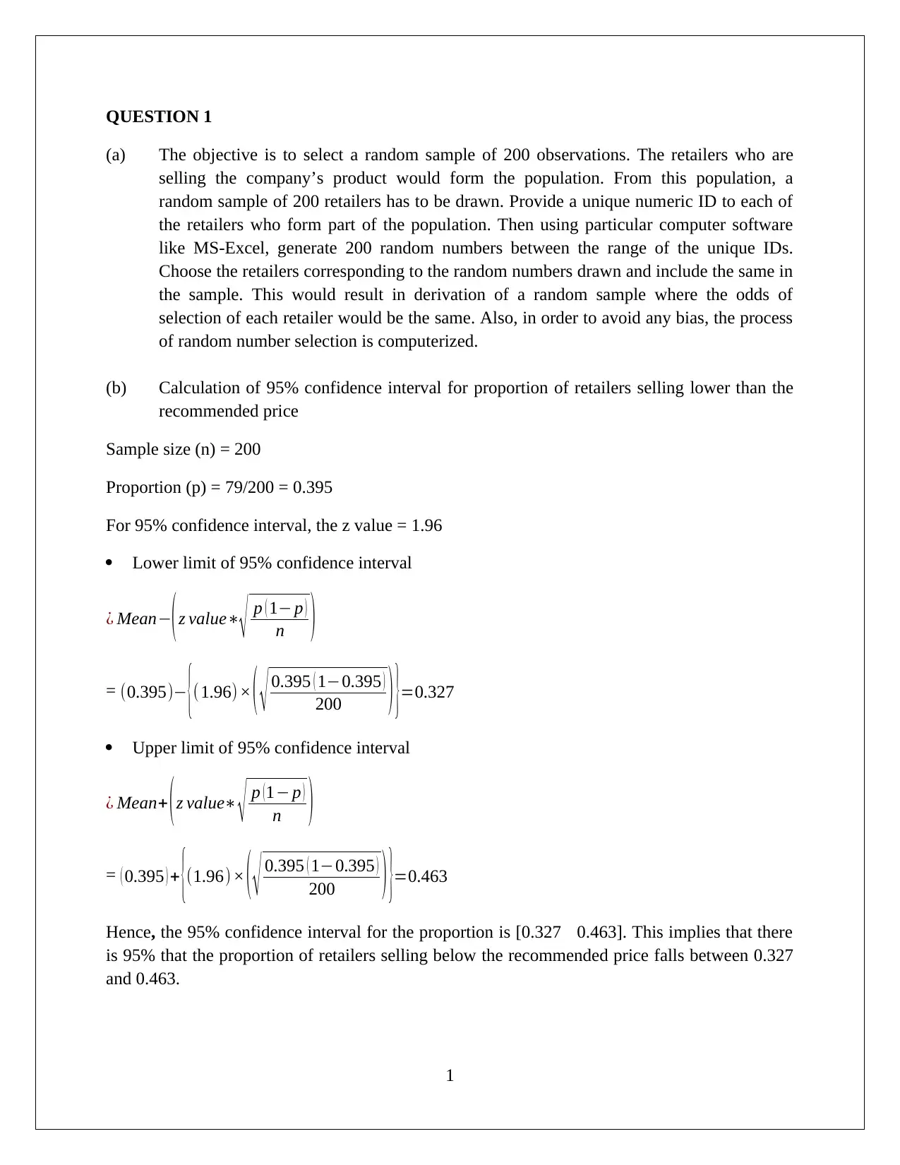
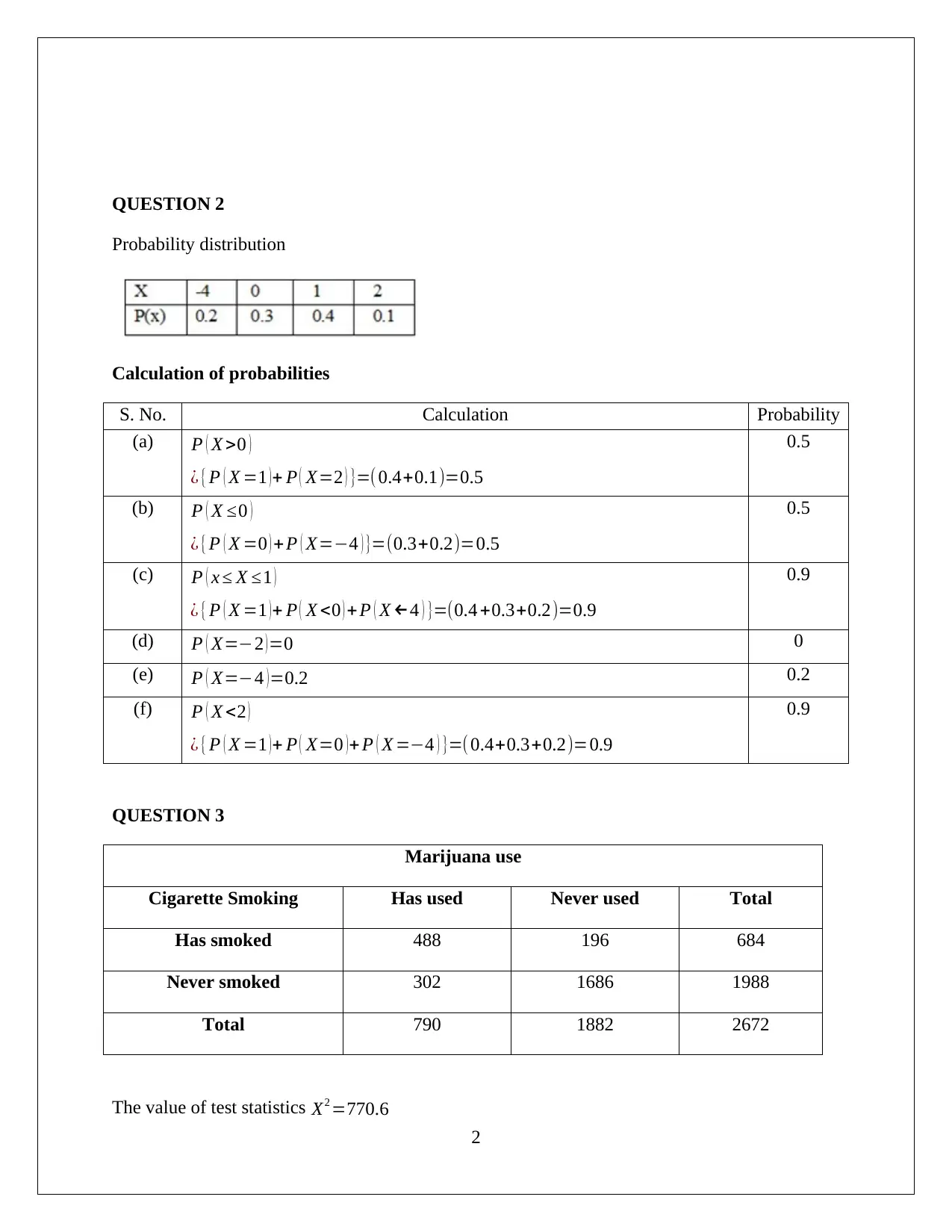
This assignment solution for QAB 105 (Quantitative Analysis for Business) covers various statistical concepts. Question 1 focuses on creating a random sample of retailers and calculating a 95% confidence interval for the proportion of retailers selling below a recommended price. Question 2 involves calculating probabilities. Question 3 explores the association between cigarette smoking and marijuana use using hypothesis testing and p-values. Question 4 investigates whether homes near a city have higher values than the mean, also employing hypothesis testing and t-statistics. Finally, Question 5 presents a linear regression model to analyze the relationship between cost and units of output, including an interpretation of the R-squared value, the significance of the slope, and the strength of the relationship based on a scatter plot and correlation coefficient.

QAB 105 Quantitative Analysis for Business
Assessment Task – 2
[Pick the date]
Student Id & Name

QUESTION 1
(a) The objective is to select a random sample of 200 observations. The retailers who are
selling the company’s product would form the population. From this population, a
random sample of 200 retailers has to be drawn. Provide a unique numeric ID to each of
the retailers who form part of the population. Then using particular computer software
like MS-Excel, generate 200 random numbers between the range of the unique IDs.
Choose the retailers corresponding to the random numbers drawn and include the same in
the sample. This would result in derivation of a random sample where the odds of
selection of each retailer would be the same. Also, in order to avoid any bias, the process
of random number selection is computerized.
(b) Calculation of 95% confidence interval for proportion of retailers selling lower than the
recommended price
Sample size (n) = 200
Proportion (p) = 79/200 = 0.395
For 95% confidence interval, the z value = 1.96
 Lower limit of 95% confidence interval
¿ Mean−( z value∗
√ p ( 1− p )
n )
= (0.395)− {(1.96) × ( √ 0.395 ( 1−0.395 )
200 ) }=0.327
 Upper limit of 95% confidence interval
¿ Mean+ ( z value∗ √ p ( 1− p )
n )
= ( 0.395 ) + {(1.96) × ( √ 0.395 ( 1−0.395 )
200 ) }=0.463
Hence, the 95% confidence interval for the proportion is [0.327 0.463]. This implies that there
is 95% that the proportion of retailers selling below the recommended price falls between 0.327
and 0.463.
1

QUESTION 2
Probability distribution
Calculation of probabilities
S. No. Calculation Probability
(a) P ( X >0 )
¿ {P ( X =1 ) + P ( X=2 ) }=( 0.4+0.1)=0.5
0.5
(b) P ( X ≤0 )
¿ {P ( X =0 ) + P ( X=−4 ) }=(0.3+0.2)=0.5
0.5
(c) P ( x ≤ X ≤1 )
¿ {P ( X =1 ) + P ( X <0 ) + P ( X ←4 ) }=(0.4 +0.3+0.2)=0.9
0.9
(d) P ( X=−2 )=0 0
(e) P ( X=−4 )=0.2 0.2
(f) P ( X <2 )
¿ {P ( X =1 ) + P ( X=0 ) + P ( X =−4 ) }=( 0.4+0.3+0.2)=0.9
0.9
QUESTION 3
Marijuana use
Cigarette Smoking Has used Never used Total
Has smoked 488 196 684
Never smoked 302 1686 1988
Total 790 1882 2672
The value of test statistics X2 =770.6
2

Step 1
The respective hypotheses are highlighted below:
Null hypothesis H0 :There is no direct association present between cigarette smoking and
marijuana.
Alternative hypothesis H1 : There is direct association present between cigarette smoking and
marijuana.
Step 2
Degree of freedom dof =( n−1)(r−1)=(2−1)∗(2−1)=1
Step 3
The p value for the test statistics X2 =770.6 and 1 degree of freedom (for two tailed) comes out
to be 0.0001.
Step 4
Assuming level of significance = 5%
Step 5
It can be seen from above that p value is lower than the level of significance (0.0001<0.05).
Therefore, significant evidence is present to reject H0 (null hypothesis) and to accept H1
(alternative hypothesis). Hence, there is direct association present between cigarette smoking and
marijuana.
QUESTION 4
The data and information is summarized below:
Level of significance ∝ = 5%
Mean value μ = $88,950
Random sample size n = 12
Mean valuation x= $92,460
Standard deviation s = $5,200
Step 1
3

The respective hypotheses are highlighted below:
Null hypothesis H0 μ=88950
Alternative hypothesis H1 : μ> 88950
Step 2
Computation of t statistics
t statistics=
( x−μ
s
√ n )
t statistics=
{ ( 92460−88950 )
( 5200
√ 12 ) }=2.338
Step 3
Degree of freedom dof = ( n−1 ) = ( 12−1 ) =11
Step 4
The p value for the test statistics t=2.338 and 11 degree of freedom (for single tailed) comes out
to be 0.00.
Step 5
It can be seen from above that p value is lower than the level of significance (0.00<0.05).
Therefore, significant evidence is present to reject H0 (null hypothesis) and to accept H1
(alternative hypothesis). Hence, homes in vicinity of the city have higher values as compared
with the mean value ($88,950).
QUESTION 5
The data and information is summarized below:
4

(a) The linear regression model for the above data is shown below:
Dependent variable - Cost ($000’)
Independent variable - Units of output (000’)
Regression equation from the above output
Cost ( $ 000' ) =21.25+ { ( Units of outputs ) ×0.9615 }
Comments: It is apparent that the R2 value is close to the theoretical maximum of 1 and hence the
model represents a good fit. Also, the slope of the independent variable is significant. Further,
5

the slope is positive which presents that there is a positive association between the given
variables of interest.
(b) The level of strength of relationship between cost and units of outputs would be decided
based on the given factors.
 By scatter plot
In the scatter plot indicated below, it is apparent that the various values tend to follow a linear
trend with very minimal deviations which is representative of the fact that the linear relationship
between the two variables is very strong.
 By correlation coefficient
The value of correlation coefficient (R) has been found with the help of R square value from
regression output.
R square = 0.9884
Correlation coefficient (R) = √0.9884 = 0.9942
6