Quantitative Analysis Assignment - Quantitative Techniques Module

This assignment solution addresses key concepts in quantitative analysis, covering topics relevant to a statistics and probability course. It begins with a differentiation between moving averages and composite averages, providing practical examples. The solution then delves into probability, including theoretical probability distributions and its application in business decision-making. Hypothesis testing, including the steps involved and the conditions of normal distribution, is also explained. Various sampling techniques, such as quota sampling, judgmental sampling, snowball sampling, and convenience sampling are discussed. Practical examples illustrate the application of these techniques. Finally, the assignment contrasts permutations and combinations, highlighting their differences and applications. The solution also includes answers to specific quantitative problems involving probability calculations. References and a bibliography are provided to support the content.

Running head: QUANTITATIVE ANALYSIS
Quantitative Analysis
Name of the Student:
Name of the University:
Author note:

1QUANTITATIVE ANALYSIS
Table of Contents
Answer to the question 1............................................................................................................2
Part (a)....................................................................................................................................2
Part (b)....................................................................................................................................3
Part (c)....................................................................................................................................4
Part (d)....................................................................................................................................4
Part (e)....................................................................................................................................5
Part (f)....................................................................................................................................6
Answer to the question 2............................................................................................................6
Part (a)....................................................................................................................................6
Part (b)....................................................................................................................................7
References and Bibliography...................................................................................................10
Answer to the question 1

2QUANTITATIVE ANALYSIS
Part (a)
(i) Moving average is an indicator of trend. It is based on past prices. It is identify the
trend or business of an economy (Wang et al. 2014). The example of moving
average is as below
Let (t1, y1), (t2, y2), …, (tn, yn) denote a time series. Where y1, y2, …, yn are the values of the
variable y; corresponding to time periods t1, t2, …, tn. For order m the moving average is
y1+y2+……+ym / m and the next one is y2+……+ym+ ym+1 / m.
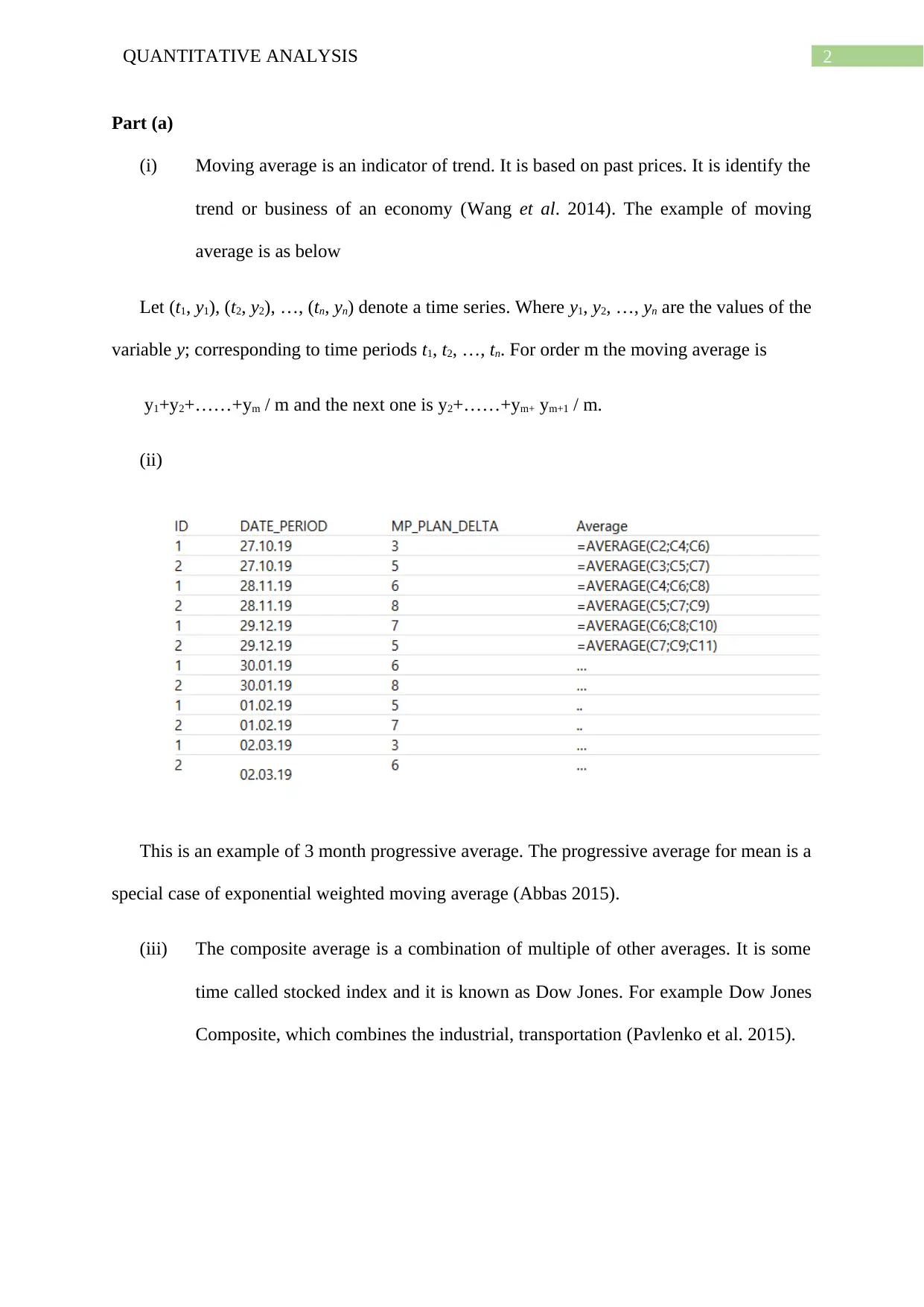
(ii)
This is an example of 3 month progressive average. The progressive average for mean is a
special case of exponential weighted moving average (Abbas 2015).
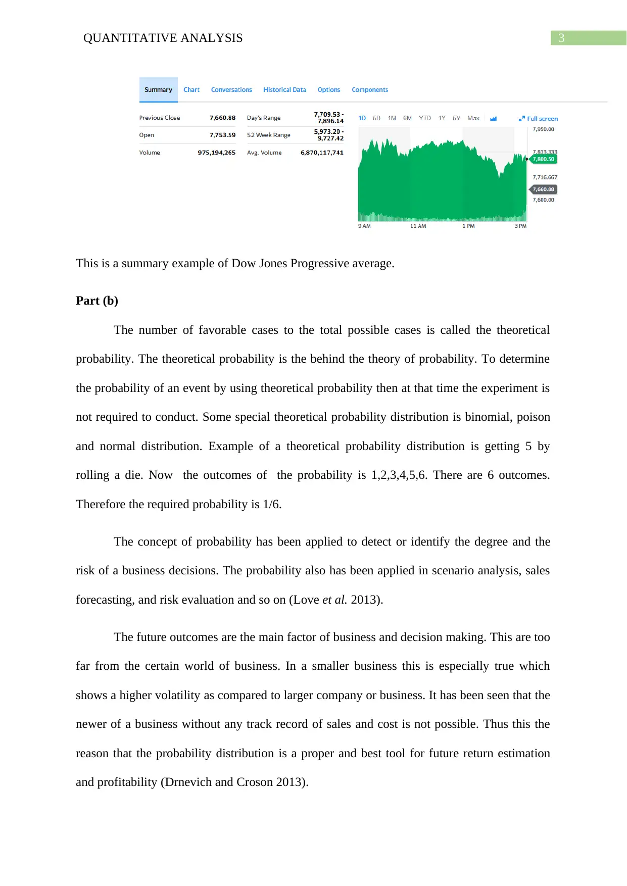
(iii) The composite average is a combination of multiple of other averages. It is some
time called stocked index and it is known as Dow Jones. For example Dow Jones
Composite, which combines the industrial, transportation (Pavlenko et al. 2015).

3QUANTITATIVE ANALYSIS
This is a summary example of Dow Jones Progressive average.
Part (b)
The number of favorable cases to the total possible cases is called the theoretical
probability. The theoretical probability is the behind the theory of probability. To determine
the probability of an event by using theoretical probability then at that time the experiment is
not required to conduct. Some special theoretical probability distribution is binomial, poison
and normal distribution. Example of a theoretical probability distribution is getting 5 by
rolling a die. Now the outcomes of the probability is 1,2,3,4,5,6. There are 6 outcomes.
Therefore the required probability is 1/6.
The concept of probability has been applied to detect or identify the degree and the
risk of a business decisions. The probability also has been applied in scenario analysis, sales
forecasting, and risk evaluation and so on (Love et al. 2013).
The future outcomes are the main factor of business and decision making. This are too
far from the certain world of business. In a smaller business this is especially true which
shows a higher volatility as compared to larger company or business. It has been seen that the
newer of a business without any track record of sales and cost is not possible. Thus this the
reason that the probability distribution is a proper and best tool for future return estimation
and profitability (Drnevich and Croson 2013).

4QUANTITATIVE ANALYSIS
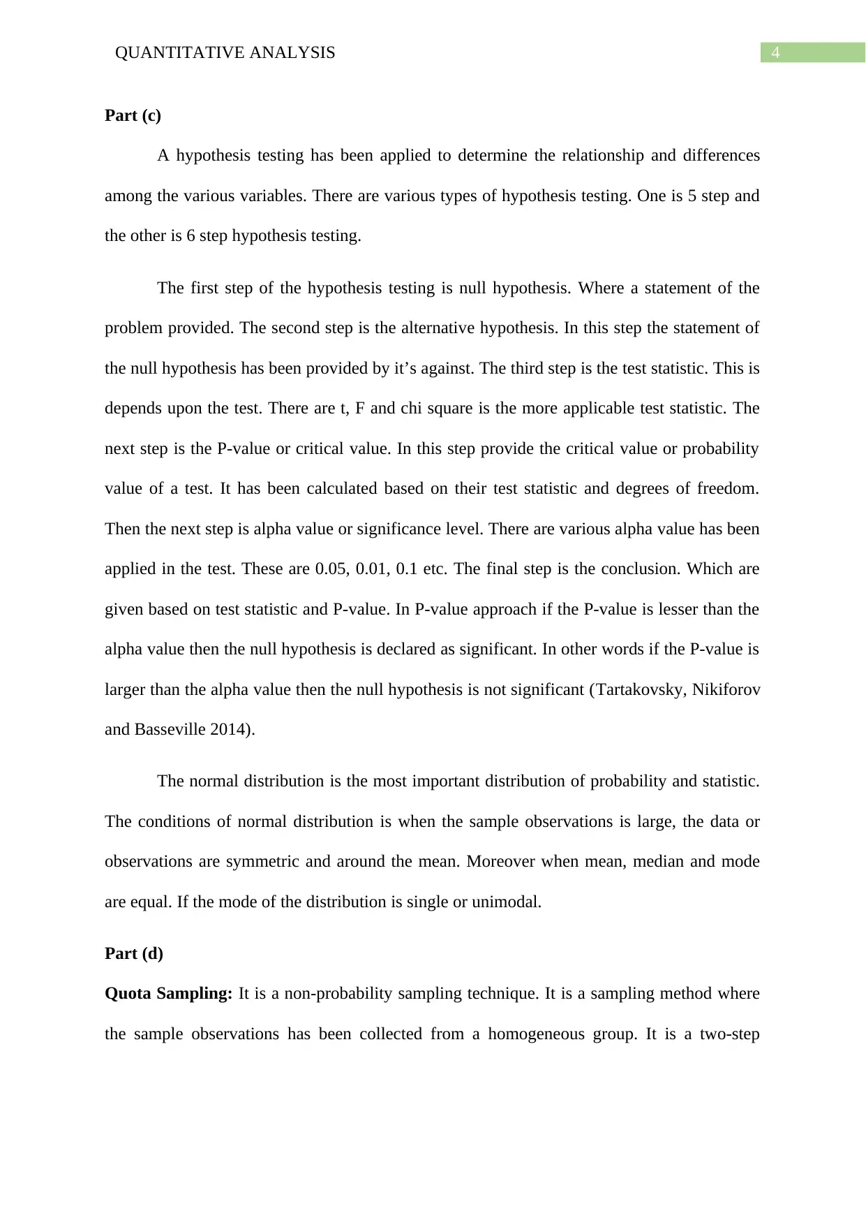
Part (c)
A hypothesis testing has been applied to determine the relationship and differences
among the various variables. There are various types of hypothesis testing. One is 5 step and
the other is 6 step hypothesis testing.
The first step of the hypothesis testing is null hypothesis. Where a statement of the
problem provided. The second step is the alternative hypothesis. In this step the statement of
the null hypothesis has been provided by it’s against. The third step is the test statistic. This is
depends upon the test. There are t, F and chi square is the more applicable test statistic. The
next step is the P-value or critical value. In this step provide the critical value or probability
value of a test. It has been calculated based on their test statistic and degrees of freedom.
Then the next step is alpha value or significance level. There are various alpha value has been
applied in the test. These are 0.05, 0.01, 0.1 etc. The final step is the conclusion. Which are
given based on test statistic and P-value. In P-value approach if the P-value is lesser than the
alpha value then the null hypothesis is declared as significant. In other words if the P-value is
larger than the alpha value then the null hypothesis is not significant (Tartakovsky, Nikiforov
and Basseville 2014).
The normal distribution is the most important distribution of probability and statistic.
The conditions of normal distribution is when the sample observations is large, the data or
observations are symmetric and around the mean. Moreover when mean, median and mode
are equal. If the mode of the distribution is single or unimodal.
Part (d)
Quota Sampling: It is a non-probability sampling technique. It is a sampling method where
the sample observations has been collected from a homogeneous group. It is a two-step

5QUANTITATIVE ANALYSIS
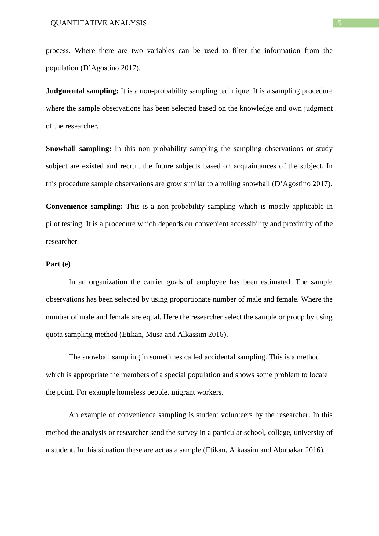
process. Where there are two variables can be used to filter the information from the
population (D’Agostino 2017).
Judgmental sampling: It is a non-probability sampling technique. It is a sampling procedure
where the sample observations has been selected based on the knowledge and own judgment
of the researcher.
Snowball sampling: In this non probability sampling the sampling observations or study
subject are existed and recruit the future subjects based on acquaintances of the subject. In
this procedure sample observations are grow similar to a rolling snowball (D’Agostino 2017).
Convenience sampling: This is a non-probability sampling which is mostly applicable in
pilot testing. It is a procedure which depends on convenient accessibility and proximity of the
researcher.
Part (e)
In an organization the carrier goals of employee has been estimated. The sample
observations has been selected by using proportionate number of male and female. Where the
number of male and female are equal. Here the researcher select the sample or group by using
quota sampling method (Etikan, Musa and Alkassim 2016).
The snowball sampling in sometimes called accidental sampling. This is a method
which is appropriate the members of a special population and shows some problem to locate
the point. For example homeless people, migrant workers.
An example of convenience sampling is student volunteers by the researcher. In this
method the analysis or researcher send the survey in a particular school, college, university of
a student. In this situation these are act as a sample (Etikan, Alkassim and Abubakar 2016).

6QUANTITATIVE ANALYSIS
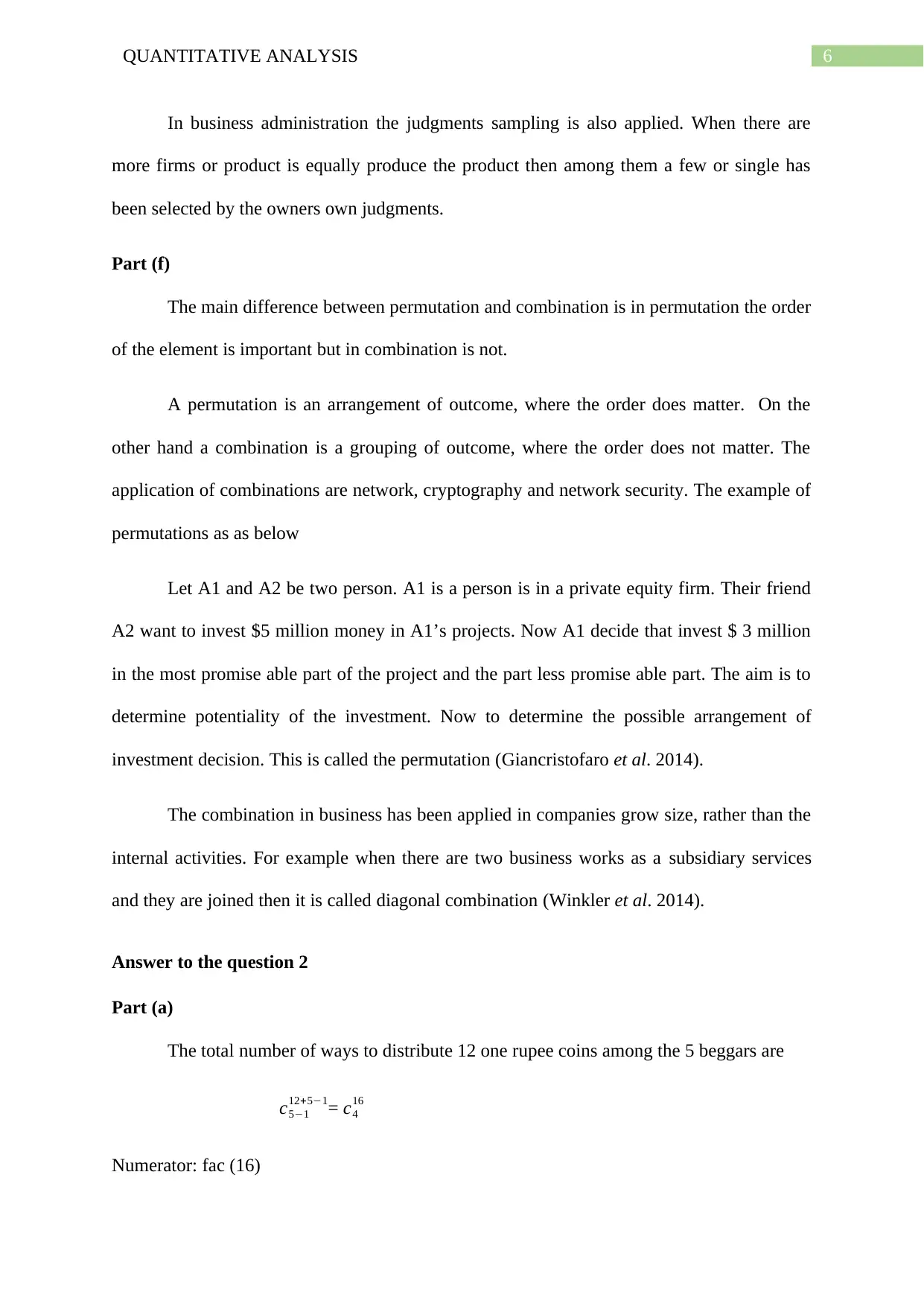
In business administration the judgments sampling is also applied. When there are
more firms or product is equally produce the product then among them a few or single has
been selected by the owners own judgments.
Part (f)
The main difference between permutation and combination is in permutation the order
of the element is important but in combination is not.
A permutation is an arrangement of outcome, where the order does matter. On the
other hand a combination is a grouping of outcome, where the order does not matter. The
application of combinations are network, cryptography and network security. The example of
permutations as as below
Let A1 and A2 be two person. A1 is a person is in a private equity firm. Their friend
A2 want to invest $5 million money in A1’s projects. Now A1 decide that invest $ 3 million
in the most promise able part of the project and the part less promise able part. The aim is to
determine potentiality of the investment. Now to determine the possible arrangement of
investment decision. This is called the permutation (Giancristofaro et al. 2014).
The combination in business has been applied in companies grow size, rather than the
internal activities. For example when there are two business works as a subsidiary services
and they are joined then it is called diagonal combination (Winkler et al. 2014).
Answer to the question 2
Part (a)
The total number of ways to distribute 12 one rupee coins among the 5 beggars are
c5−1
12+5−1= c4
16
Numerator: fac (16)

7QUANTITATIVE ANALYSIS
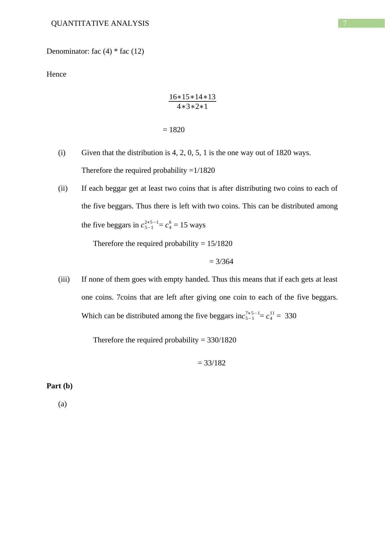
Denominator: fac (4) * fac (12)
Hence
16∗15∗14∗13
4∗3∗2∗1
= 1820
(i) Given that the distribution is 4, 2, 0, 5, 1 is the one way out of 1820 ways.
Therefore the required probability =1/1820
(ii) If each beggar get at least two coins that is after distributing two coins to each of
the five beggars. Thus there is left with two coins. This can be distributed among
the five beggars in c5−1
2+5 −1= c4
6 = 15 ways
Therefore the required probability = 15/1820
= 3/364
(iii) If none of them goes with empty handed. Thus this means that if each gets at least
one coins. 7coins that are left after giving one coin to each of the five beggars.
Which can be distributed among the five beggars inc5−1
7+ 5−1= c4
11 = 330
Therefore the required probability = 330/1820
= 33/182
Part (b)
(a)

8QUANTITATIVE ANALYSIS
(b)
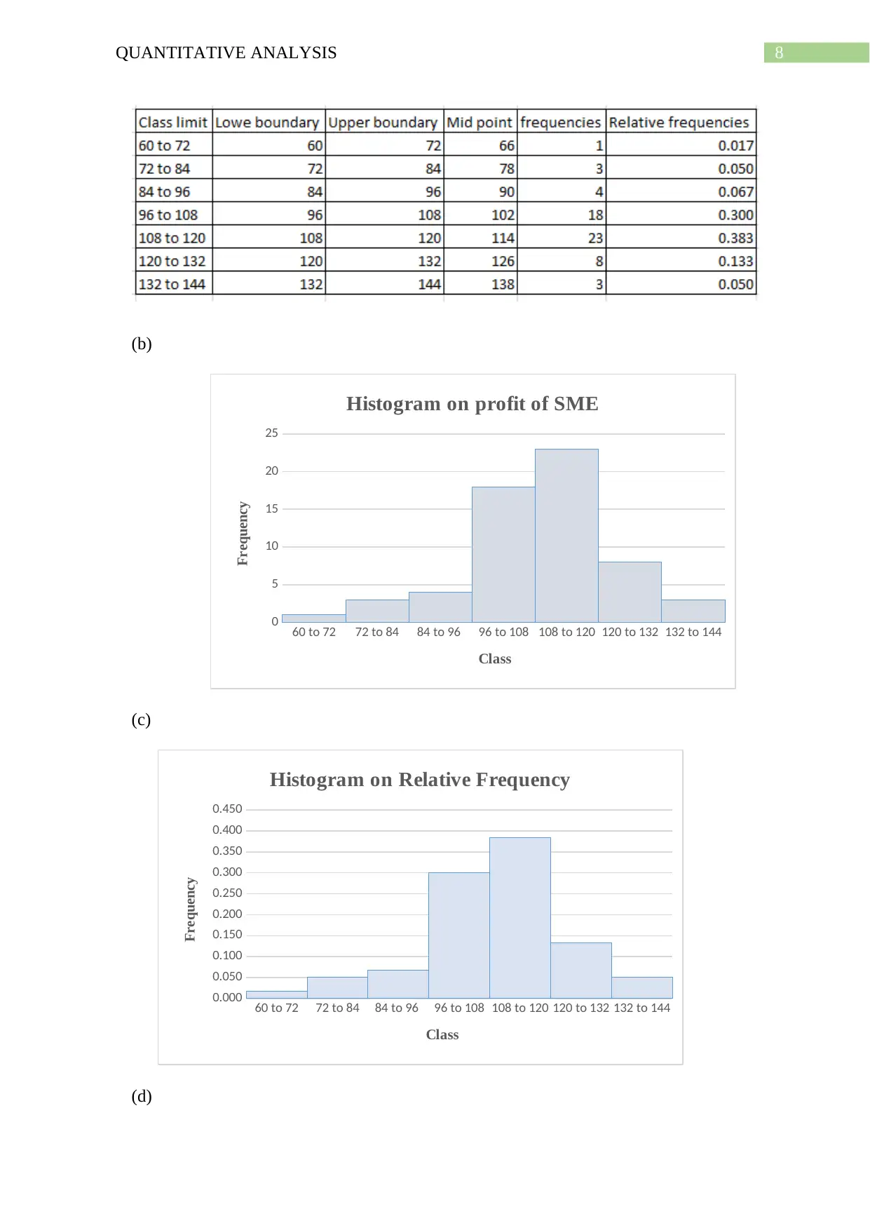
60 to 72 72 to 84 84 to 96 96 to 108 108 to 120 120 to 132 132 to 144
0
5
10
15
20
25
Histogram on profit of SME
Class
Frequency
(c)
60 to 72 72 to 84 84 to 96 96 to 108 108 to 120 120 to 132 132 to 144
0.000
0.050
0.100
0.150
0.200
0.250
0.300
0.350
0.400
0.450
Histogram on Relative Frequency
Class
Frequency
(d)

9QUANTITATIVE ANALYSIS
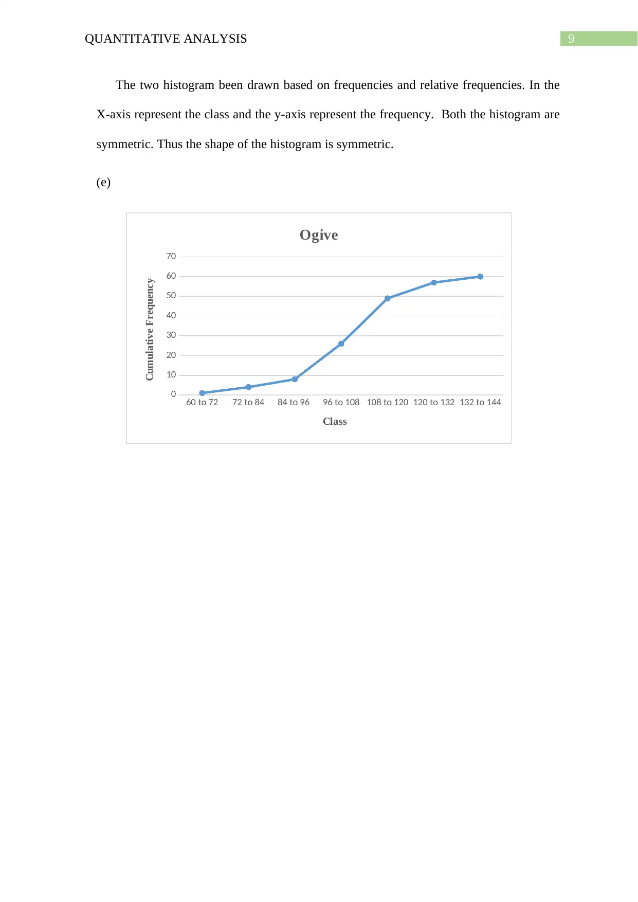
The two histogram been drawn based on frequencies and relative frequencies. In the
X-axis represent the class and the y-axis represent the frequency. Both the histogram are
symmetric. Thus the shape of the histogram is symmetric.
(e)
60 to 72 72 to 84 84 to 96 96 to 108 108 to 120 120 to 132 132 to 144
0
10
20
30
40
50
60
70
Ogive
Class
Cumulative Frequency

10QUANTITATIVE ANALYSIS
References and Bibliography
Abbas, N., 2015. Progressive mean as a special case of exponentially weighted moving
average. Quality and Reliability Engineering International, 31(4), pp.719-720.
Amato, M.S., Boyle, R.G. and Levy, D., 2016. How to define e-cigarette prevalence? Finding
clues in the use frequency distribution. Tobacco control, 25(e1), pp.e24-e29.
D’Agostino, R.B., 2017. Tests for the normal distribution. In Goodness-of-fit-techniques (pp.
367-420). Routledge.
Drnevich, P.L. and Croson, D.C., 2013. Information technology and business-level strategy:
toward an integrated theoretical perspective. Mis Quarterly, pp.483-509.
Etikan, I., Alkassim, R. and Abubakar, S., 2016. Comparision of snowball sampling and
sequential sampling technique. Biometrics and Biostatistics International Journal, 3(1), p.55.
Etikan, I., Musa, S.A. and Alkassim, R.S., 2016. Comparison of convenience sampling and
purposive sampling. American journal of theoretical and applied statistics, 5(1), pp.1-4.
Giancristofaro, R.A., Carrozzo, E., Cichi, I., Boatto, V. and Barisan, L., 2014. The influence
of the dependency structure in combination-based multivariate permutation tests in case of
ordered categorical responses. In Topics in Statistical Simulation (pp. 229-238). Springer,
New York, NY.
Gnedenko, B.V., 2018. Theory of probability. Routledge.
Groebner, D.F., Shannon, P.W., Fry, P.C. and Smith, K.D., 2013. Business statistics. Pearson
Education UK.
Love, P.E., Sing, C.P., Wang, X., Edwards, D.J. and Odeyinka, H., 2013. Probability
distribution fitting of schedule overruns in construction projects. Journal of the Operational
Research Society, 64(8), pp.1231-1247.

11QUANTITATIVE ANALYSIS
Michael, G.G., 2013. Planetary surface dating from crater size–frequency distribution
measurements: Multiple resurfacing episodes and differential isochron fitting. Icarus, 226(1),
pp.885-890.
Pavlenko, V.I., Cherkashina, N.I., Yastrebinskij, R.N. and Noskov, A.V., 2015. The
theoretical calculation of the average mileage of electrons of energies up to 10 MeV in
polymer composite. Voprosy Atomnoj Nauki i Tekhniki, pp.32-35.
Tartakovsky, A., Nikiforov, I. and Basseville, M., 2014. Sequential analysis: Hypothesis
testing and changepoint detection. CRC Press.
Wang, J., Liang, J., Gao, F., Zhang, L. and Wang, Z., 2014. A method to improve the
dynamic performance of moving average filter-based PLL. IEEE Transactions on Power
Electronics, 30(10), pp.5978-5990.
Winkler, A.M., Ridgway, G.R., Webster, M.A., Smith, S.M. and Nichols, T.E., 2014.
Permutation inference for the general linear model. Neuroimage, 92, pp.381-397.