Quantitative Methods for Business: Statistical Analysis Assignment

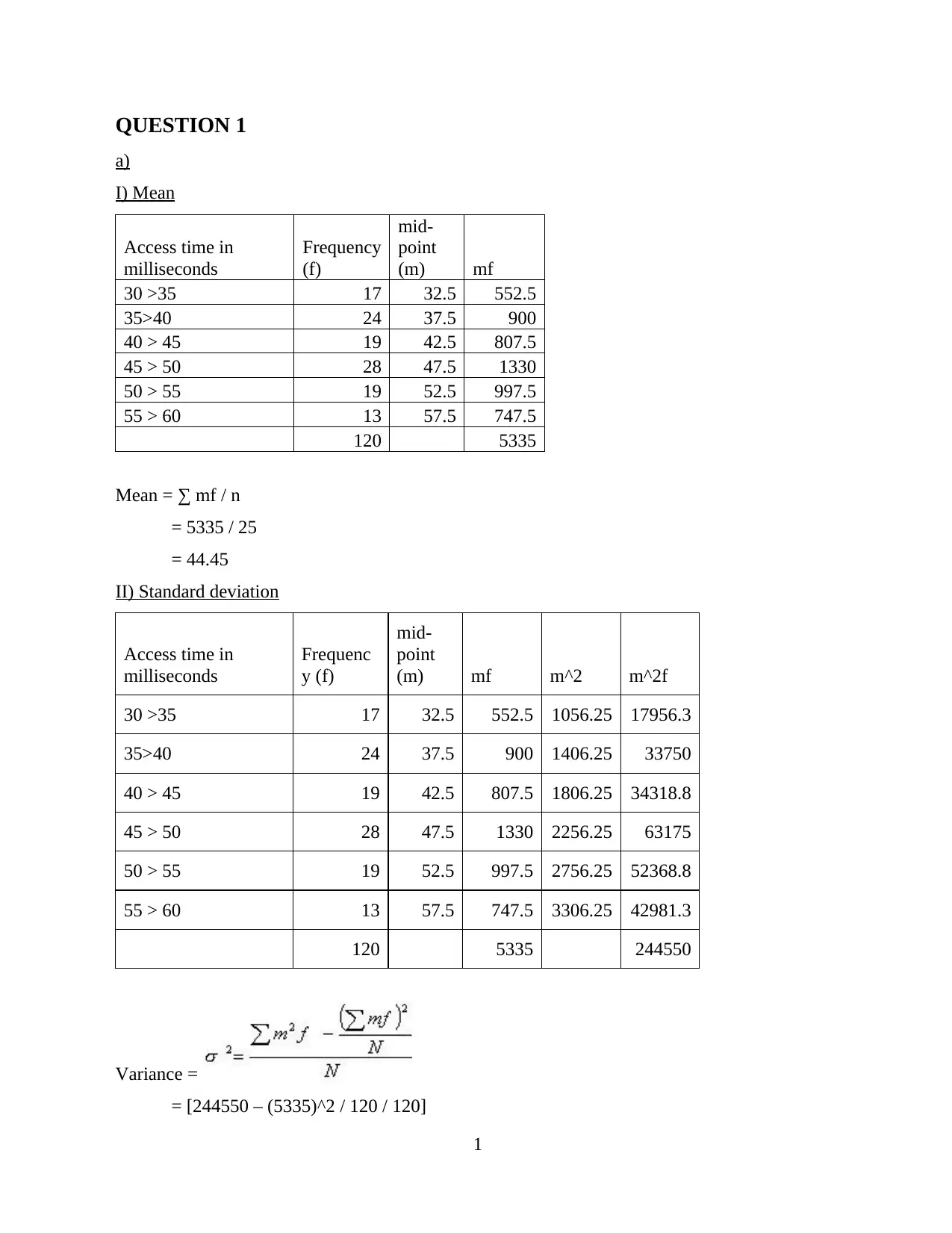
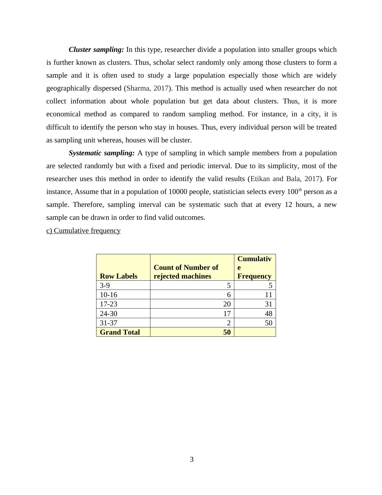
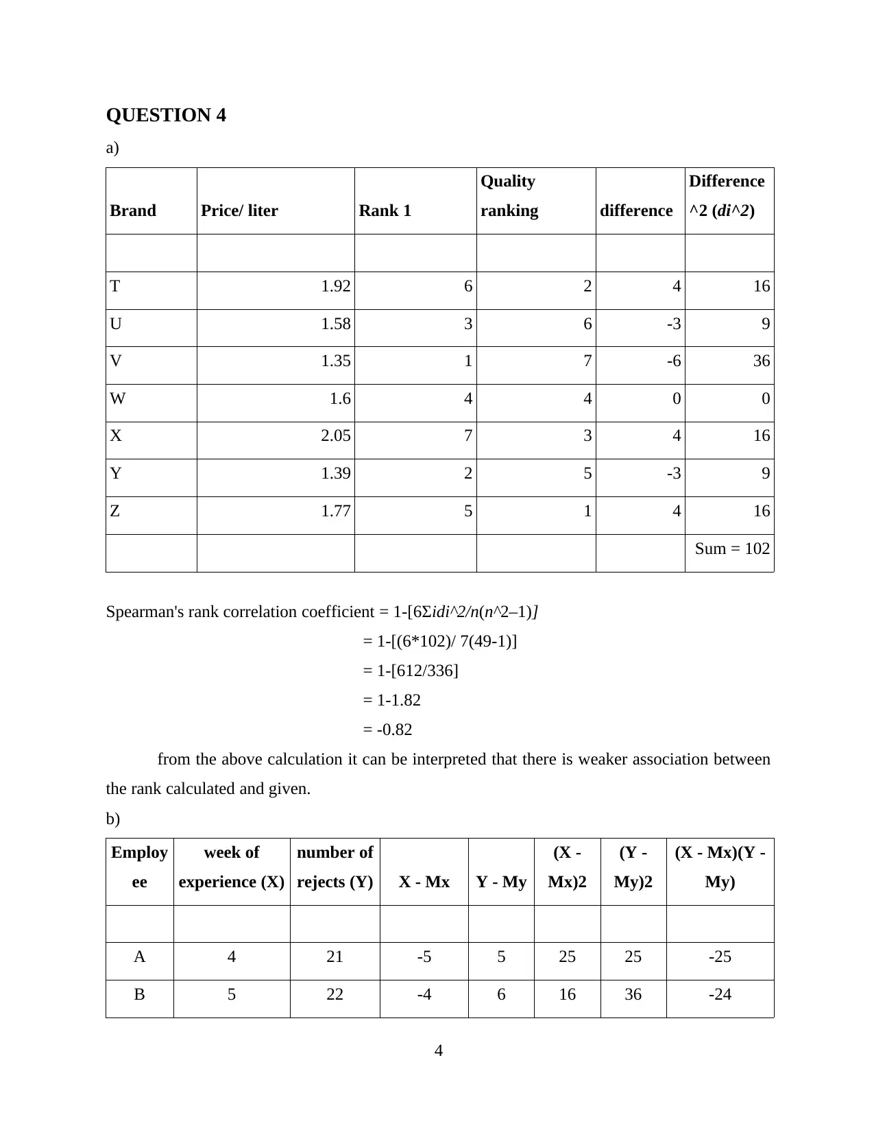
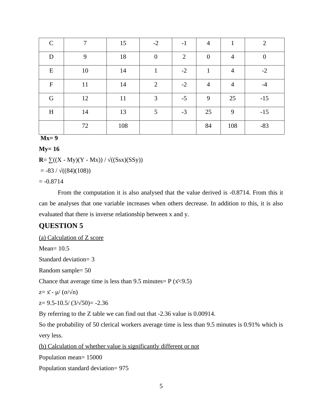
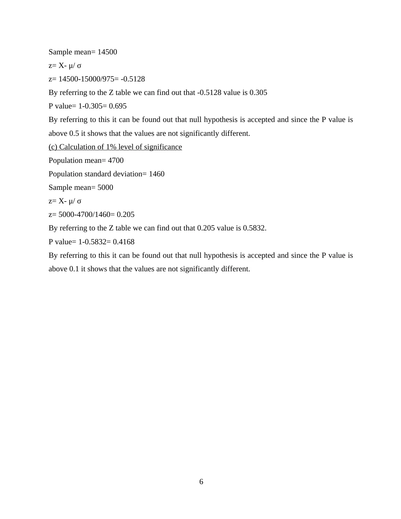
This assignment delves into quantitative methods used in a business context, covering several key areas of statistical analysis. The solution begins with the calculation and interpretation of the mean and standard deviation from a frequency distribution table, demonstrating how to analyze data related to access time in a computer disc system. It then explores different sampling methods, including simple random sampling, quota sampling, cluster sampling, and systematic sampling, with examples illustrating their application. The assignment continues with the calculation of cumulative frequency. Further analysis includes the calculation of Spearman's rank correlation coefficient and the interpretation of the relationship between variables. Finally, the assignment concludes with the calculation of Z-scores and P-values to determine statistical significance, including examples related to clerical worker average time and population mean comparisons, providing a comprehensive overview of statistical techniques relevant to business analysis.

Quantitative methods for
business alternative

Table of Contents
QUESTION 1...................................................................................................................................1
a)..................................................................................................................................................1
I) Mean........................................................................................................................................1
II) Standard deviation..................................................................................................................1
III) Interpret the results...............................................................................................................2
b) Sampling methods...................................................................................................................2
c) Cumulative frequency.............................................................................................................3
QUESTION 4...................................................................................................................................4
QUESTION 5...................................................................................................................................5
(a) Calculation of Z score............................................................................................................5
(b) Calculation of whether value is significantly different or not...............................................5
(c) Calculation of 1% level of significance.................................................................................6
REFERENCES................................................................................................................................7

QUESTION 1
a)
I) Mean
Access time in
milliseconds
Frequency
(f)
mid-
point
(m) mf
30 >35 17 32.5 552.5
35>40 24 37.5 900
40 > 45 19 42.5 807.5
45 > 50 28 47.5 1330
50 > 55 19 52.5 997.5
55 > 60 13 57.5 747.5
120 5335
Mean = ∑ mf / n
= 5335 / 25
= 44.45
II) Standard deviation
Access time in
milliseconds
Frequenc
y (f)
mid-
point
(m) mf m^2 m^2f
30 >35 17 32.5 552.5 1056.25 17956.3
35>40 24 37.5 900 1406.25 33750
40 > 45 19 42.5 807.5 1806.25 34318.8
45 > 50 28 47.5 1330 2256.25 63175
50 > 55 19 52.5 997.5 2756.25 52368.8
55 > 60 13 57.5 747.5 3306.25 42981.3
120 5335 244550
Variance =
= [244550 – (5335)^2 / 120 / 120]
1

= [244550 – 237185.2]/ 120
= 7364.79/ 120
= 61.37
Standard deviation = under-root of variance
= √61.37
= 7.83
III) Interpret the results
Through the table, it is interpreted that average time required to made computer disc
system is 44.45. Whereas, the value of standard deviation indicates 7.83 which means that
around 7.83 milliseconds are required to dispersed the data in relation to defined mean.
b) Sampling methods
Simple random sampling: It is a type of probability sampling in which scholar randomly
selected some participants from a population. In this, each member of a population has an equal
chance to participate within selected data (Cai and et.al., 2019). With the help of this data,
researcher did not find any mistakes and provide valid results as well. For example, To identify
the working culture of a company, manager uses simple random sampling method in which 20
employees are randomly selected out of 300 population. In this, company's manager collect the
reviews by asking relevant questions pertaining to organization culture and draw valid results as
well. Further, company made appropriate actions, if find any negative results. Thus, it is
analyzed that with this method, researcher save time and money in order to gain valid outputs.
Quota sampling: It is a type of non-probability sampling method in which researcher
chooses sample as per specific traits or qualities. The main reason for using this sampling is
such that it allows researcher to sample a subgroup as per the interest (Ochoa and Porcar, 2018).
This method is considered an ideal technique for researchers because sample are chosen as per
the their characteristics. For example, To identify the career goal of University students among
fresher, junior and senior. There are 10000 students and it is considered as a population. So,
there were 3000 fresher (30%), 2500 juniors (25%) and 2000 senior (20%). It reflects that
having a sample of 1000 students then researcher has to considered 300 freshers, 250 juniors and
200 seniors as per the quota sampling
2

Cluster sampling: In this type, researcher divide a population into smaller groups which
is further known as clusters. Thus, scholar select randomly only among those clusters to form a
sample and it is often used to study a large population especially those which are widely
geographically dispersed (Sharma, 2017). This method is actually used when researcher do not
collect information about whole population but get data about clusters. Thus, it is more
economical method as compared to random sampling method. For instance, in a city, it is
difficult to identify the person who stay in houses. Thus, every individual person will be treated
as sampling unit whereas, houses will be cluster.
Systematic sampling: A type of sampling in which sample members from a population
are selected randomly but with a fixed and periodic interval. Due to its simplicity, most of the
researcher uses this method in order to identify the valid results (Etikan and Bala, 2017). For
instance, Assume that in a population of 10000 people, statistician selects every 100th person as a
sample. Therefore, sampling interval can be systematic such that at every 12 hours, a new
sample can be drawn in order to find valid outcomes.
c) Cumulative frequency
Row Labels
Count of Number of
rejected machines
Cumulativ
e
Frequency
3-9 5 5
10-16 6 11
17-23 20 31
24-30 17 48
31-37 2 50
Grand Total 50
3

QUESTION 4
a)
Brand Price/ liter Rank 1
Quality
ranking difference
Difference
^2 (di^2)
T 1.92 6 2 4 16
U 1.58 3 6 -3 9
V 1.35 1 7 -6 36
W 1.6 4 4 0 0
X 2.05 7 3 4 16
Y 1.39 2 5 -3 9
Z 1.77 5 1 4 16
Sum = 102
Spearman's rank correlation coefficient = 1-[6Σidi^2/n(n^2–1)]
= 1-[(6*102)/ 7(49-1)]
= 1-[612/336]
= 1-1.82
= -0.82
from the above calculation it can be interpreted that there is weaker association between
the rank calculated and given.
b)
Employ
ee
week of
experience (X)
number of
rejects (Y) X - Mx Y - My
(X -
Mx)2
(Y -
My)2
(X - Mx)(Y -
My)
A 4 21 -5 5 25 25 -25
B 5 22 -4 6 16 36 -24
4

C 7 15 -2 -1 4 1 2
D 9 18 0 2 0 4 0
E 10 14 1 -2 1 4 -2
F 11 14 2 -2 4 4 -4
G 12 11 3 -5 9 25 -15
H 14 13 5 -3 25 9 -15
72 108 84 108 -83
Mx= 9
My= 16
R= ∑((X - My)(Y - Mx)) / √((Ssx)(SSy))
= -83 / √((84)(108))
= -0.8714
From the computation it is also analysed that the value derived is -0.8714. From this it
can be analyses that one variable increases when others decrease. In addition to this, it is also
evaluated that there is inverse relationship between x and y.
QUESTION 5
(a) Calculation of Z score
Mean= 10.5
Standard deviation= 3
Random sample= 50
Chance that average time is less than 9.5 minutes= P (x̄<9.5)
z= x̄ - μ/ (σ/√n)
z= 9.5-10.5/ (3/√50)= -2.36
By referring to the Z table we can find out that -2.36 value is 0.00914.
So the probability of 50 clerical workers average time is less than 9.5 minutes is 0.91% which is
very less.
(b) Calculation of whether value is significantly different or not
Population mean= 15000
Population standard deviation= 975
5

Sample mean= 14500
z= X- μ/ σ
z= 14500-15000/975= -0.5128
By referring to the Z table we can find out that -0.5128 value is 0.305
P value= 1-0.305= 0.695
By referring to this it can be found out that null hypothesis is accepted and since the P value is
above 0.5 it shows that the values are not significantly different.
(c) Calculation of 1% level of significance
Population mean= 4700
Population standard deviation= 1460
Sample mean= 5000
z= X- μ/ σ
z= 5000-4700/1460= 0.205
By referring to the Z table we can find out that 0.205 value is 0.5832.
P value= 1-0.5832= 0.4168
By referring to this it can be found out that null hypothesis is accepted and since the P value is
above 0.1 it shows that the values are not significantly different.
6

REFERENCES
Books and Journals
Cai, S. and et.al., 2019. Empirical likelihood confidence intervals under imputation for missing
survey data from stratified simple random sampling. Canadian Journal of Statistics.
47(2). pp.281-301.
Etikan, I. and Bala, K., 2017. Sampling and sampling methods. Biometrics & Biostatistics
International Journal. 5(6). p.00149.
Ochoa, C. and Porcar, J. M., 2018. Modeling the effect of quota sampling on online fieldwork
efficiency: An analysis of the connection between uncertainty and sample
usage. International Journal of Market Research. 60(5). pp.484-501.
Sharma, G., 2017. Pros and cons of different sampling techniques. International journal of
applied research. 3(7). pp.749-752.
7