Quantitative Business Analysis: Income and Expenditure Analysis

This report provides a quantitative business analysis focusing on the relationship between take-home pay and weekly food expenditure. It utilizes statistical methods such as frequency distribution, histograms, and regression analysis to determine the correlation between these two variables. The analysis reveals a strong positive correlation, indicating that as take-home pay increases, so does weekly food expenditure. The report includes detailed tables and figures illustrating the data and regression statistics, ultimately concluding that weekly take-home pay is a significant predictor of weekly food expenditure. The study also discusses the skewness of the data distributions and suggests that larger sample sizes and inclusion of more variables could enhance future research.

Running Head: QUANTITTAIVE BUSINESS ANALYSIS
Quantitative Business Analysis
Name of the student:
Name of the university:
Course ID:

1QUANTITTAIVE BUSINESS ANALYSIS
Table of Contents
Part 1................................................................................................................................................2
1. a)...............................................................................................................................................2
1. b)..............................................................................................................................................2
1. c)...............................................................................................................................................2
Part 2................................................................................................................................................2
2. a)...............................................................................................................................................2
2. b)..............................................................................................................................................3
2. c)...............................................................................................................................................4
2. d)..............................................................................................................................................6
Part 3................................................................................................................................................6
3. a)...............................................................................................................................................6
3. b)..............................................................................................................................................6
3. c)...............................................................................................................................................7
3. d)..............................................................................................................................................7
3. e)...............................................................................................................................................8
Part 4................................................................................................................................................8
References:....................................................................................................................................10

2QUANTITTAIVE BUSINESS ANALYSIS
Table of Tables
Table 1: Frequency distribution of take-home pay..........................................................................5
Table 2: Frequency distribution of weekly food expenditure..........................................................5
Table 3: Numerical summary of ‘Take-home pay’ and ‘Weekly food expenditure’......................6
Table 4: Table of regression statistics.............................................................................................9
Table 5: Table of regression coefficients and ANOVA table of simple linear regression............10
Table of Figures
Figure 1: Histogram of take-home pay............................................................................................4
Figure 2: Histogram of weekly-food expenditure...........................................................................5
Figure 3: Scatter plot of ‘Weekly Food Expenditure ($)’ and ‘Take-home pay ($)’......................8

3QUANTITTAIVE BUSINESS ANALYSIS
Part 1.
1. a)
The researchers could have utilized ‘Mail survey’ (by survey questionnaire) for collecting
data. The method is less time taking, cheap and the surveyor may frame his/her questions as per
his/her requirement (Ansolabehere and Schaffner 2014, pp.285-303). A huge amount of data
could be gathered or collected by this process in short duration.
1. b)
The researchers could use the most popular probabilistic sampling method that is ‘Simple
random sampling’ to select the sample from the entire population. As it is processed by
randomization method, therefore, the probability of occurrence of bias would be very
insignificant.
1. c)
The major issue that researchers may face in this collection is that- unavailability of email
ids of huge amount of people. The response rate is always uncertain in the considered process.
Also, absence of direct communication between surveyor and responders might lead to data set
that includes deliberate or undeliberate biases and errors.
Part 2.

4QUANTITTAIVE BUSINESS ANALYSIS
2. a)
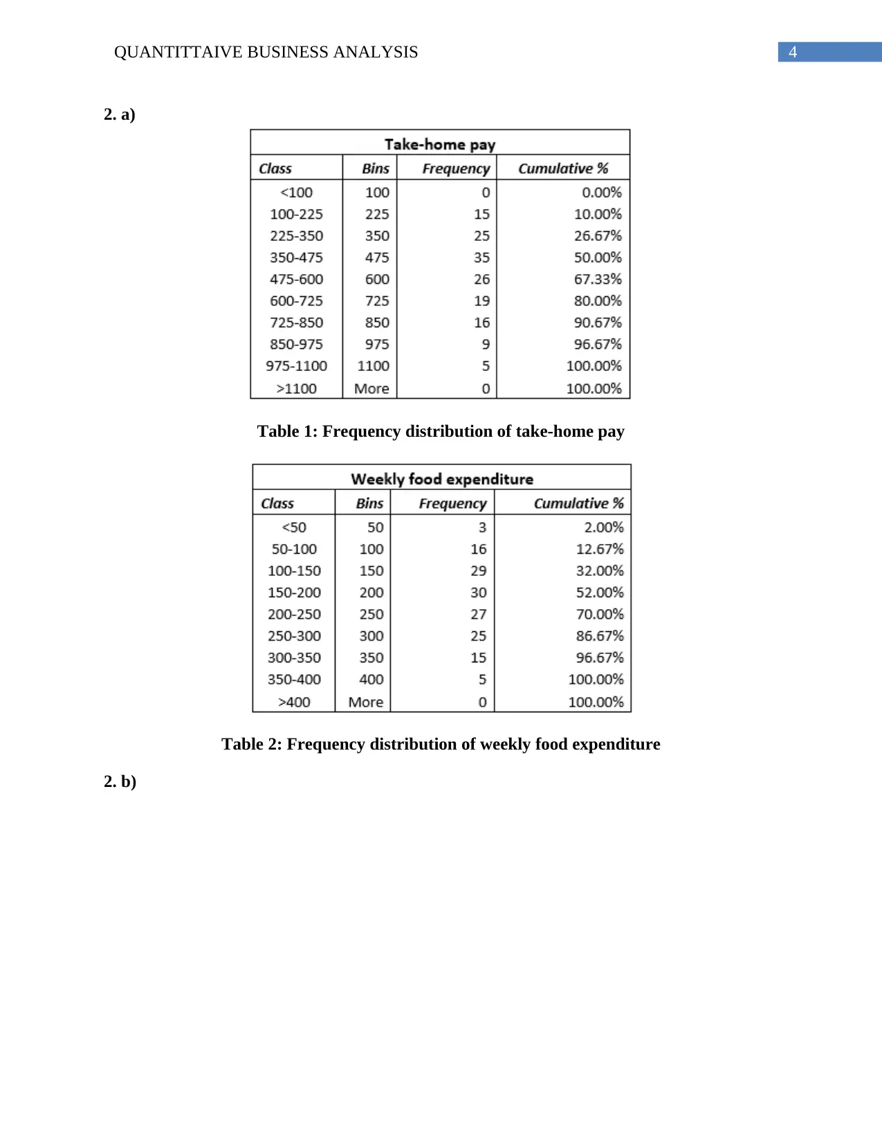
Table 1: Frequency distribution of take-home pay
Table 2: Frequency distribution of weekly food expenditure
2. b)

5QUANTITTAIVE BUSINESS ANALYSIS
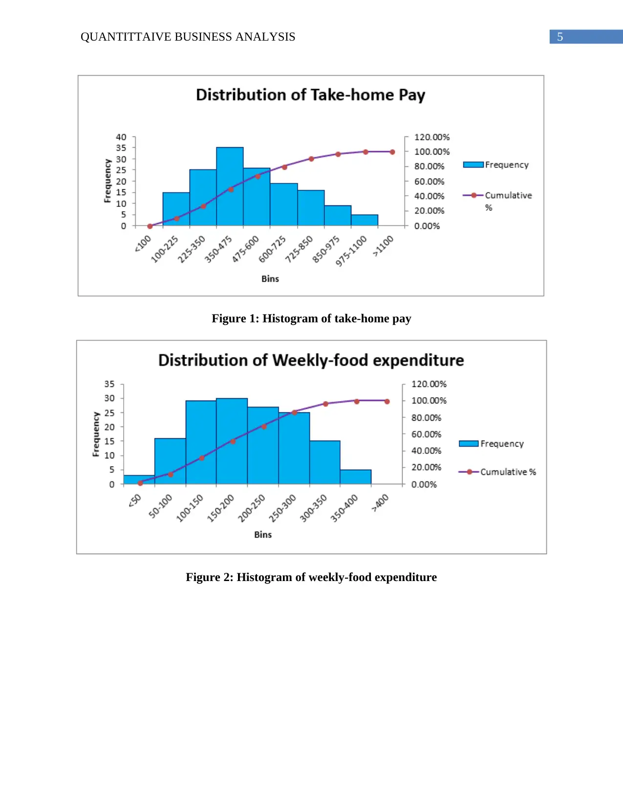
Figure 1: Histogram of take-home pay
Figure 2: Histogram of weekly-food expenditure

6QUANTITTAIVE BUSINESS ANALYSIS
2. c)
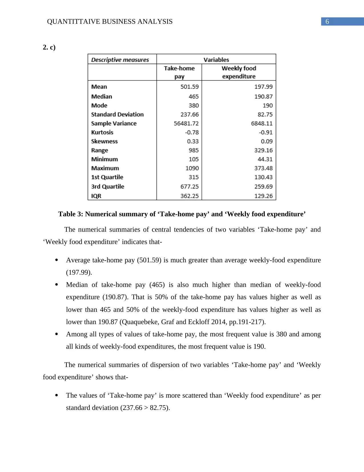
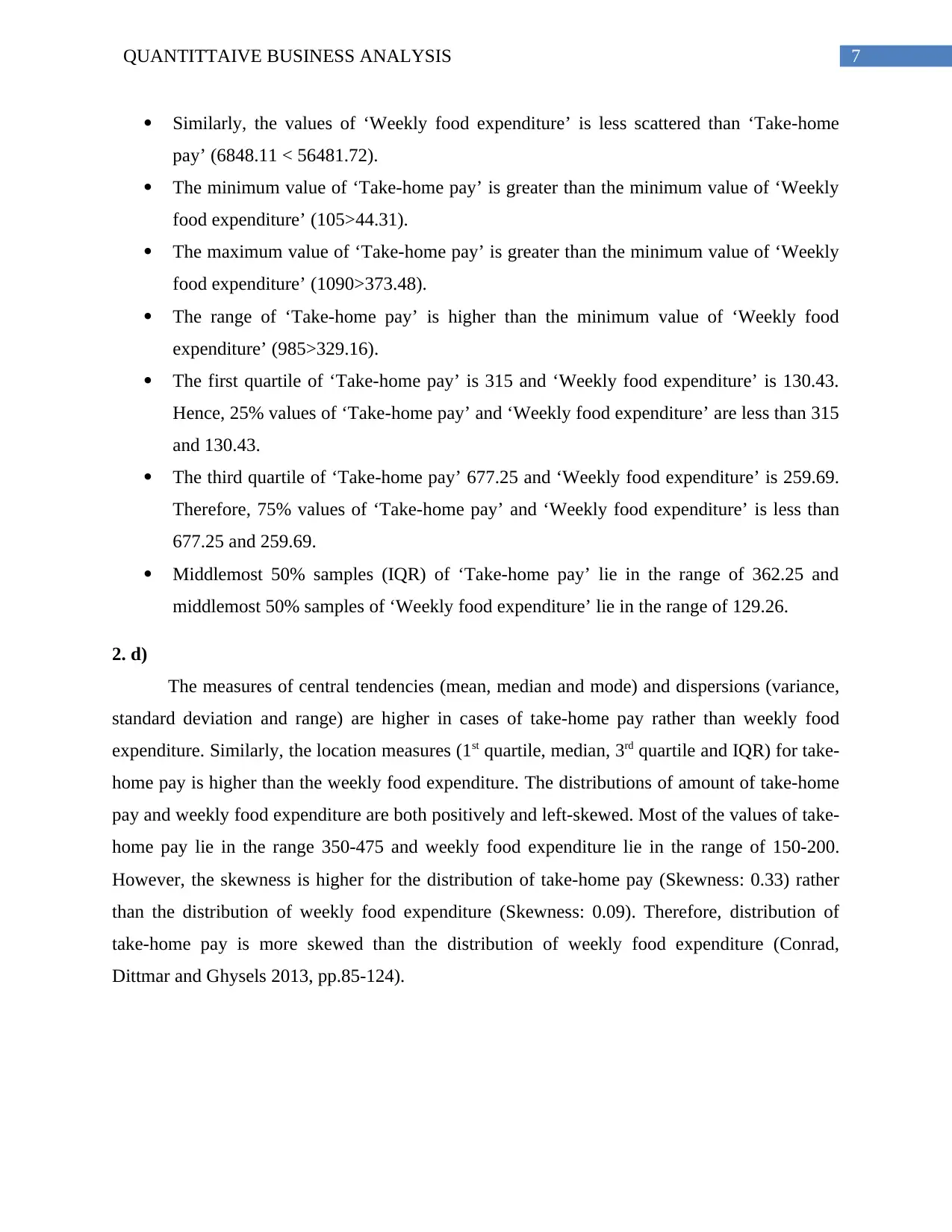
Table 3: Numerical summary of ‘Take-home pay’ and ‘Weekly food expenditure’
The numerical summaries of central tendencies of two variables ‘Take-home pay’ and
‘Weekly food expenditure’ indicates that-
 Average take-home pay (501.59) is much greater than average weekly-food expenditure
(197.99).
 Median of take-home pay (465) is also much higher than median of weekly-food
expenditure (190.87). That is 50% of the take-home pay has values higher as well as
lower than 465 and 50% of the weekly-food expenditure has values higher as well as
lower than 190.87 (Quaquebeke, Graf and Eckloff 2014, pp.191-217).
 Among all types of values of take-home pay, the most frequent value is 380 and among
all kinds of weekly-food expenditures, the most frequent value is 190.
The numerical summaries of dispersion of two variables ‘Take-home pay’ and ‘Weekly
food expenditure’ shows that-
 The values of ‘Take-home pay’ is more scattered than ‘Weekly food expenditure’ as per
standard deviation (237.66 > 82.75).

7QUANTITTAIVE BUSINESS ANALYSIS
 Similarly, the values of ‘Weekly food expenditure’ is less scattered than ‘Take-home
pay’ (6848.11 < 56481.72).
 The minimum value of ‘Take-home pay’ is greater than the minimum value of ‘Weekly
food expenditure’ (105>44.31).
 The maximum value of ‘Take-home pay’ is greater than the minimum value of ‘Weekly
food expenditure’ (1090>373.48).
 The range of ‘Take-home pay’ is higher than the minimum value of ‘Weekly food
expenditure’ (985>329.16).
 The first quartile of ‘Take-home pay’ is 315 and ‘Weekly food expenditure’ is 130.43.
Hence, 25% values of ‘Take-home pay’ and ‘Weekly food expenditure’ are less than 315
and 130.43.
 The third quartile of ‘Take-home pay’ 677.25 and ‘Weekly food expenditure’ is 259.69.
Therefore, 75% values of ‘Take-home pay’ and ‘Weekly food expenditure’ is less than
677.25 and 259.69.
 Middlemost 50% samples (IQR) of ‘Take-home pay’ lie in the range of 362.25 and
middlemost 50% samples of ‘Weekly food expenditure’ lie in the range of 129.26.
2. d)
The measures of central tendencies (mean, median and mode) and dispersions (variance,
standard deviation and range) are higher in cases of take-home pay rather than weekly food
expenditure. Similarly, the location measures (1st quartile, median, 3rd quartile and IQR) for take-
home pay is higher than the weekly food expenditure. The distributions of amount of take-home
pay and weekly food expenditure are both positively and left-skewed. Most of the values of take-
home pay lie in the range 350-475 and weekly food expenditure lie in the range of 150-200.
However, the skewness is higher for the distribution of take-home pay (Skewness: 0.33) rather
than the distribution of weekly food expenditure (Skewness: 0.09). Therefore, distribution of
take-home pay is more skewed than the distribution of weekly food expenditure (Conrad,
Dittmar and Ghysels 2013, pp.85-124).

8QUANTITTAIVE BUSINESS ANALYSIS
Part 3.
3. a)
The independent variable or predictor variable (X) of the data set is ‘Take-home pay’ and
the dependent variable or response variable (Y) of the data set is ‘Weekly food expenditure’ in
this simple linear regression model.
3. b)
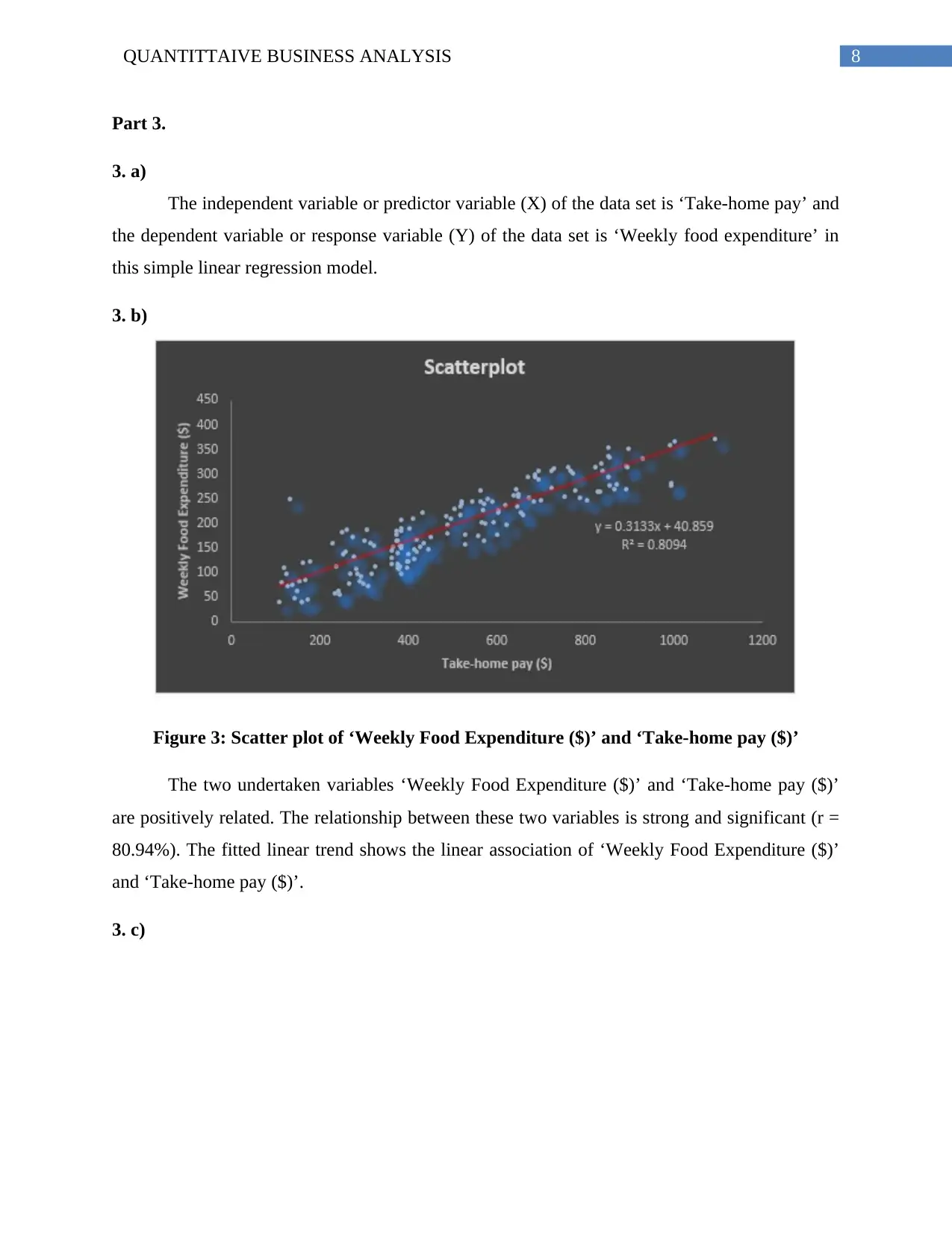
Figure 3: Scatter plot of ‘Weekly Food Expenditure ($)’ and ‘Take-home pay ($)’
The two undertaken variables ‘Weekly Food Expenditure ($)’ and ‘Take-home pay ($)’
are positively related. The relationship between these two variables is strong and significant (r =
80.94%). The fitted linear trend shows the linear association of ‘Weekly Food Expenditure ($)’
and ‘Take-home pay ($)’.
3. c)

9QUANTITTAIVE BUSINESS ANALYSIS
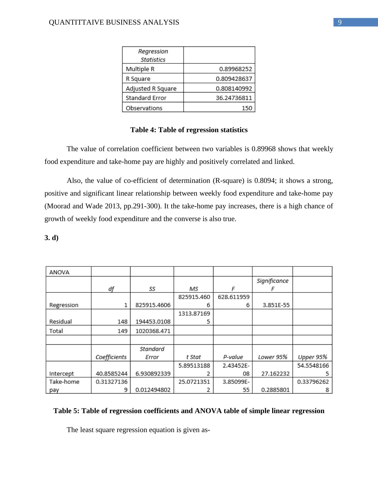
Table 4: Table of regression statistics
The value of correlation coefficient between two variables is 0.89968 shows that weekly
food expenditure and take-home pay are highly and positively correlated and linked.
Also, the value of co-efficient of determination (R-square) is 0.8094; it shows a strong,
positive and significant linear relationship between weekly food expenditure and take-home pay
(Moorad and Wade 2013, pp.291-300). It the take-home pay increases, there is a high chance of
growth of weekly food expenditure and the converse is also true.
3. d)
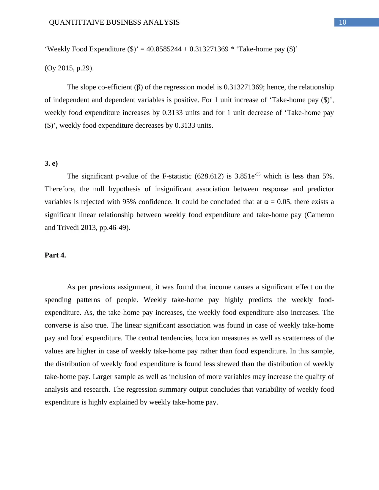
Table 5: Table of regression coefficients and ANOVA table of simple linear regression
The least square regression equation is given as-

10QUANTITTAIVE BUSINESS ANALYSIS
‘Weekly Food Expenditure ($)’ = 40.8585244 + 0.313271369 * ‘Take-home pay ($)’
(Oy 2015, p.29).
The slope co-efficient (β) of the regression model is 0.313271369; hence, the relationship
of independent and dependent variables is positive. For 1 unit increase of ‘Take-home pay ($)’,
weekly food expenditure increases by 0.3133 units and for 1 unit decrease of ‘Take-home pay
($)’, weekly food expenditure decreases by 0.3133 units.
3. e)
The significant p-value of the F-statistic (628.612) is 3.851e-55 which is less than 5%.
Therefore, the null hypothesis of insignificant association between response and predictor
variables is rejected with 95% confidence. It could be concluded that at α = 0.05, there exists a
significant linear relationship between weekly food expenditure and take-home pay (Cameron
and Trivedi 2013, pp.46-49).
Part 4.
As per previous assignment, it was found that income causes a significant effect on the
spending patterns of people. Weekly take-home pay highly predicts the weekly food-
expenditure. As, the take-home pay increases, the weekly food-expenditure also increases. The
converse is also true. The linear significant association was found in case of weekly take-home
pay and food expenditure. The central tendencies, location measures as well as scatterness of the
values are higher in case of weekly take-home pay rather than food expenditure. In this sample,
the distribution of weekly food expenditure is found less shewed than the distribution of weekly
take-home pay. Larger sample as well as inclusion of more variables may increase the quality of
analysis and research. The regression summary output concludes that variability of weekly food
expenditure is highly explained by weekly take-home pay.

11QUANTITTAIVE BUSINESS ANALYSIS
References:
Ansolabehere, S. and Schaffner, B.F., 2014. Does survey mode still matter? Findings from a
2010 multi-mode comparison. Political Analysis, 22(3), pp.285-303.
Cameron, A.C. and Trivedi, P.K., 2013. Regression analysis of count data (Vol. 53). Cambridge
university press, pp.46-49.
Conrad, J., Dittmar, R.F. and Ghysels, E., 2013. Ex ante skewness and expected stock
returns. The Journal of Finance, 68(1), pp.85-124.
Moorad, J.A. and Wade, M.J., 2013. Selection gradients, the opportunity for selection, and the
coefficient of determination. The American Naturalist, 181(3), pp.291-300.
Oy, Y., 2015. Simple linear regression. Solutions Manual for Econometrics, p.29.
Quaquebeke, N.V., Graf, M.M. and Eckloff, T., 2014. What do leaders have to live up to?
Contrasting the effects of central tendency versus ideal-based leader prototypes in leader
categorization processes. Leadership, 10(2), pp.191-217.