Quantitative Business Analytics (PMBA 6312) Final Examination

This document presents a comprehensive solution to a Quantitative Business Analytics final examination (PMBA 6312). The exam covers a range of topics, including identifying feasible regions for constraints, solving linear programming problems using the transportation model, and determining economic order quantities (EOQ). The solution includes detailed explanations, calculations, and interpretations of results, such as optimal solutions, objective function ranges, dual values, and right-hand-side ranges. Furthermore, the assignment addresses critical path analysis, determining expected durations, variances, and probabilities related to project management. The document is designed to assist students in understanding and mastering key concepts in business analytics and quantitative methods.

Quantitative Business Analytics 1
PMBA 6312. Final Examination
By
(Name of Student)
(Institutional Affiliation)
(Date of Submission)

Quantitative Business Analytics 2
Out of the following SIX questions, you are required to answer any FIVE of your choice;
each question is worth 50 points, for a total of 250 points for this exam. Don’t forget to
show all your work, either hand-written or in Excel.
Ch.7: 9
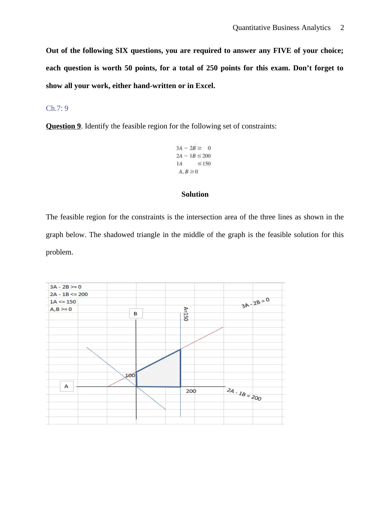
Question 9. Identify the feasible region for the following set of constraints:
Solution
The feasible region for the constraints is the intersection area of the three lines as shown in the
graph below. The shadowed triangle in the middle of the graph is the feasible solution for this
problem.

Quantitative Business Analytics 3
Ch.8: 9
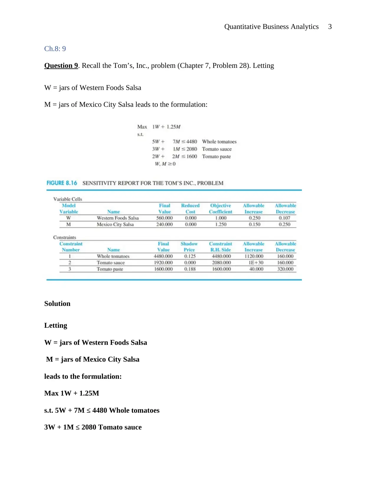
Question 9. Recall the Tom’s, Inc., problem (Chapter 7, Problem 28). Letting
W = jars of Western Foods Salsa
M = jars of Mexico City Salsa leads to the formulation:
Solution
Letting
W = jars of Western Foods Salsa
M = jars of Mexico City Salsa
leads to the formulation:
Max 1W + 1.25M
s.t. 5W + 7M ≤ 4480 Whole tomatoes
3W + 1M ≤ 2080 Tomato sauce

Quantitative Business Analytics 4
2W + 2M ≤ 1600 Tomato paste
W, M ≥ 0
The computer solution is shown in Figure 3.15.
a. What is the optimal solution, and what are the optimal production quantities?
Optimal Solution = 860
Optimal Quantities
W = 560
M=240
b. Specify the objective function ranges.
W:
Lower Limit
= 1.000 - 0.107
=0.893
Upper Limit
= 1.000 + 0.250
= 1.250
M:
Lower Limit

Quantitative Business Analytics 5
= 1.250 - 0.250
= 1.000
Upper Limit
= 1.250 + 0.150
= 1.400
c. What are the dual values for each constraint? Interpret each.
Dual Values:
Whole Tomatoes = 0.125
Tomato Sauce = 0.000
Tomato Paste = 0.1875
The values of whole tomatoes and tomato paste are Non-Zero. Hence, they are Binding
Constrains. Changing these values will change the optimal solution.
The Constraint Sauce is Zero. This is a Non-Binding Constraint. Changing this will not
have an effect on the Optimal Solution
d. Identify each of the right-hand-side ranges.
Whole Tomatoes:
Lower Limit:
= 4480 - 160
= 4320
Upper Limit:
= 4480 + 1120

Quantitative Business Analytics 6
= 5600
Tomato Sauce:
Lower Limit:
= 2080 - 160
= 1920
Upper Limit:
= 2080 + 1E + 30
= 1E + 30
Tomato Paste:
Lower Limit:
= 1600 - 320
= 1280
Upper Limit:
= 1600 + 40
= 1640
Ch.10: 9
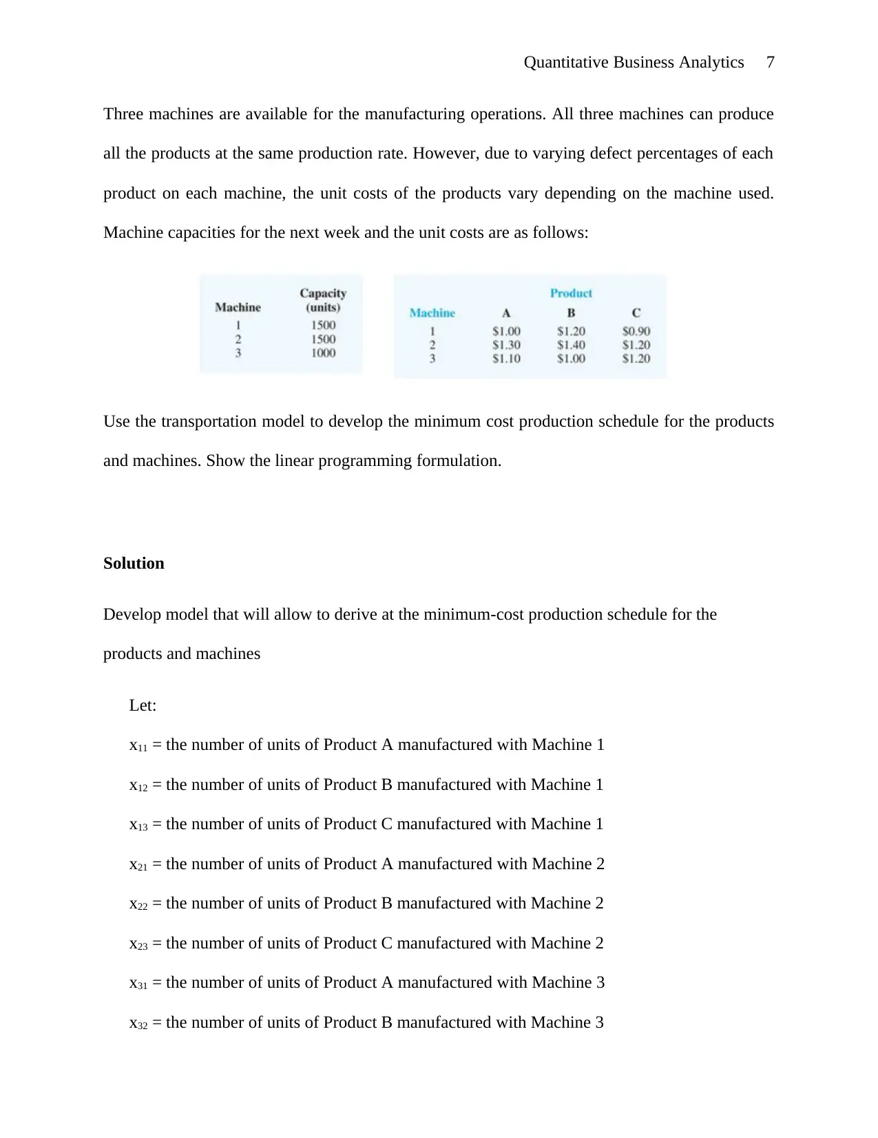
Question 9. The Ace Manufacturing Company has orders for three similar products:

Quantitative Business Analytics 7
Three machines are available for the manufacturing operations. All three machines can produce
all the products at the same production rate. However, due to varying defect percentages of each
product on each machine, the unit costs of the products vary depending on the machine used.
Machine capacities for the next week and the unit costs are as follows:
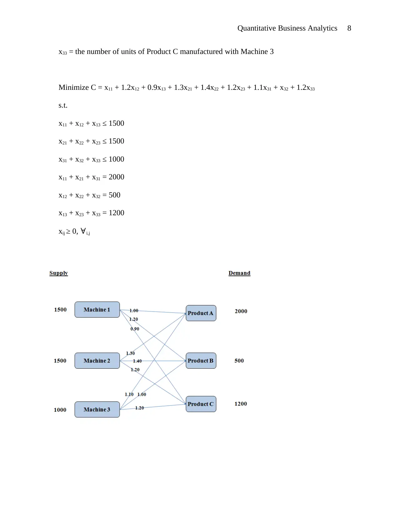
Use the transportation model to develop the minimum cost production schedule for the products
and machines. Show the linear programming formulation.
Solution
Develop model that will allow to derive at the minimum-cost production schedule for the
products and machines
Let:
x11 = the number of units of Product A manufactured with Machine 1
x12 = the number of units of Product B manufactured with Machine 1
x13 = the number of units of Product C manufactured with Machine 1
x21 = the number of units of Product A manufactured with Machine 2
x22 = the number of units of Product B manufactured with Machine 2
x23 = the number of units of Product C manufactured with Machine 2
x31 = the number of units of Product A manufactured with Machine 3
x32 = the number of units of Product B manufactured with Machine 3

Quantitative Business Analytics 8
x33 = the number of units of Product C manufactured with Machine 3
Minimize C = x11 + 1.2x12 + 0.9x13 + 1.3x21 + 1.4x22 + 1.2x23 + 1.1x31 + x32 + 1.2x33
s.t.
x11 + x12 + x13 ≤ 1500
x21 + x22 + x23 ≤ 1500
x31 + x32 + x33 ≤ 1000
x11 + x21 + x31 = 2000
x12 + x22 + x32 = 500
x13 + x23 + x33 = 1200
xij ≥ 0, ∀i,j

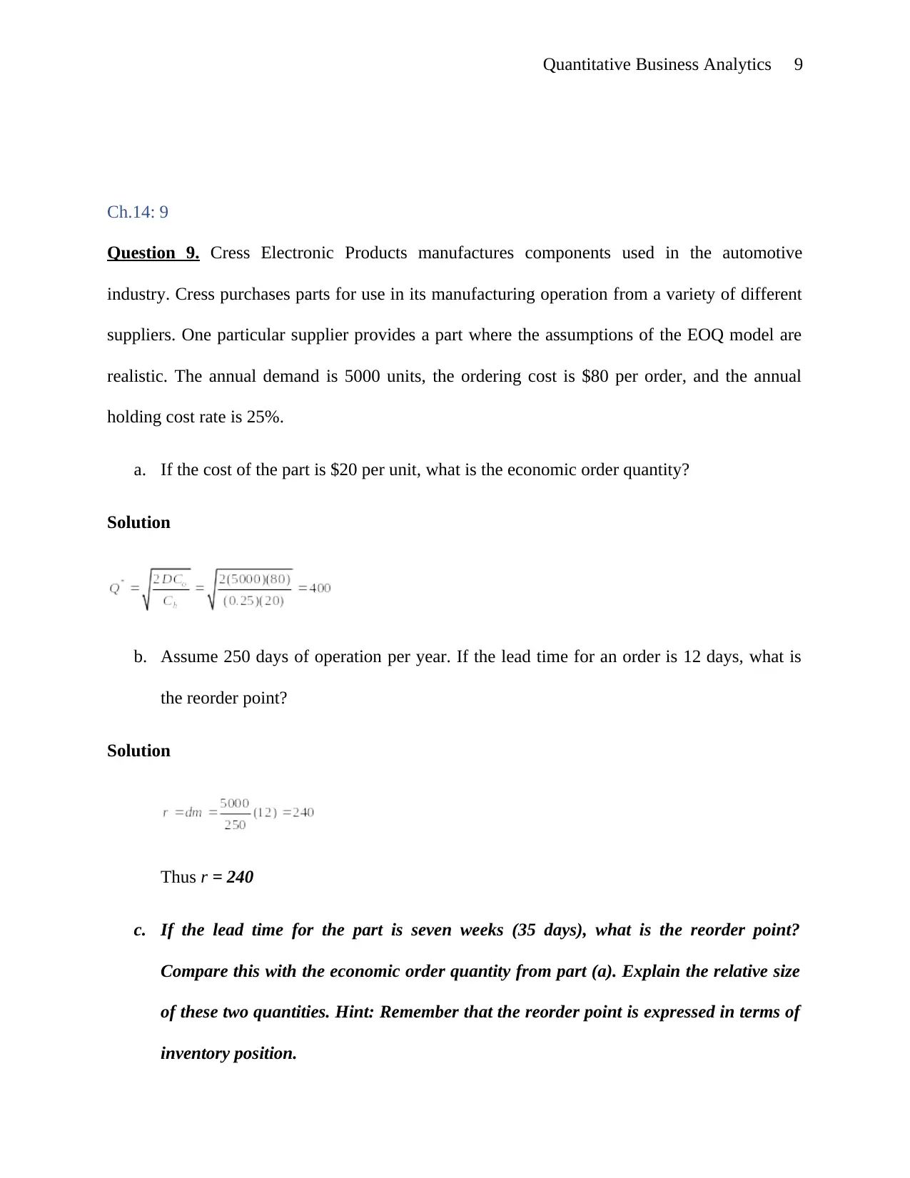
Quantitative Business Analytics 9
Ch.14: 9
Question 9. Cress Electronic Products manufactures components used in the automotive
industry. Cress purchases parts for use in its manufacturing operation from a variety of different
suppliers. One particular supplier provides a part where the assumptions of the EOQ model are
realistic. The annual demand is 5000 units, the ordering cost is $80 per order, and the annual
holding cost rate is 25%.
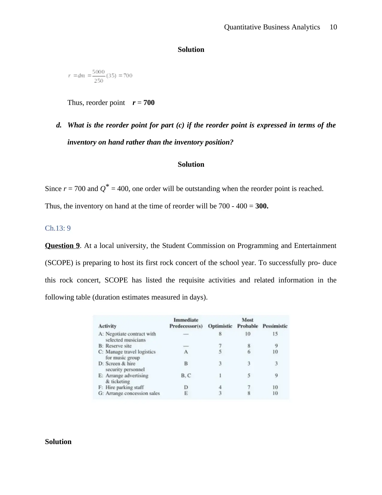
a. If the cost of the part is $20 per unit, what is the economic order quantity?
Solution
b. Assume 250 days of operation per year. If the lead time for an order is 12 days, what is
the reorder point?
Solution
Thus r = 240
c. If the lead time for the part is seven weeks (35 days), what is the reorder point?
Compare this with the economic order quantity from part (a). Explain the relative size
of these two quantities. Hint: Remember that the reorder point is expressed in terms of
inventory position.

Quantitative Business Analytics 10
Solution
Thus, reorder point r = 700
d. What is the reorder point for part (c) if the reorder point is expressed in terms of the
inventory on hand rather than the inventory position?
Solution
Since r = 700 and Q* = 400, one order will be outstanding when the reorder point is reached.
Thus, the inventory on hand at the time of reorder will be 700 - 400 = 300.
Ch.13: 9
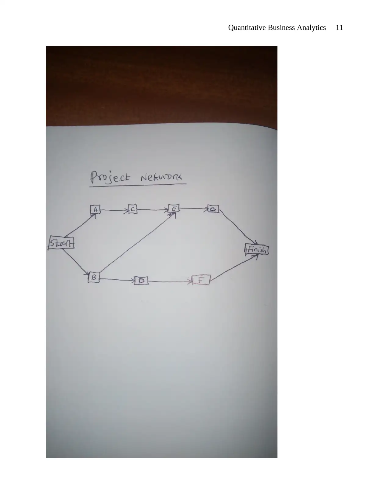
Question 9. At a local university, the Student Commission on Programming and Entertainment
(SCOPE) is preparing to host its first rock concert of the school year. To successfully pro- duce
this rock concert, SCOPE has listed the requisite activities and related information in the
following table (duration estimates measured in days).
Solution

Quantitative Business Analytics 11

Quantitative Business Analytics 12
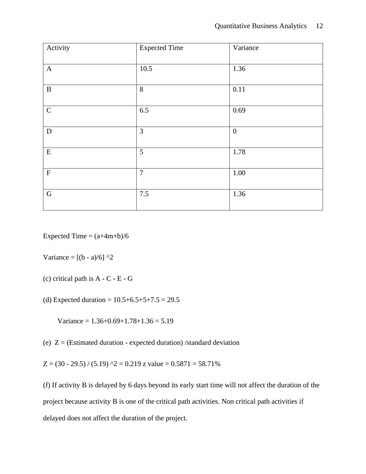
Activity Expected Time Variance
A 10.5 1.36
B 8 0.11
C 6.5 0.69
D 3 0
E 5 1.78
F 7 1.00
G 7.5 1.36
Expected Time = (a+4m+b)/6
Variance = [(b - a)/6] ^2
(c) critical path is A - C - E - G
(d) Expected duration = 10.5+6.5+5+7.5 = 29.5
Variance = 1.36+0.69+1.78+1.36 = 5.19
(e) Z = (Estimated duration - expected duration) /standard deviation
Z = (30 - 29.5) / (5.19) ^2 = 0.219 z value = 0.5871 = 58.71%
(f) If activity B is delayed by 6 days beyond its early start time will not affect the duration of the
project because activity B is one of the critical path activities. Non critical path activities if
delayed does not affect the duration of the project.