Statistics Report: Statistical Analysis of Quantitative Data, Results

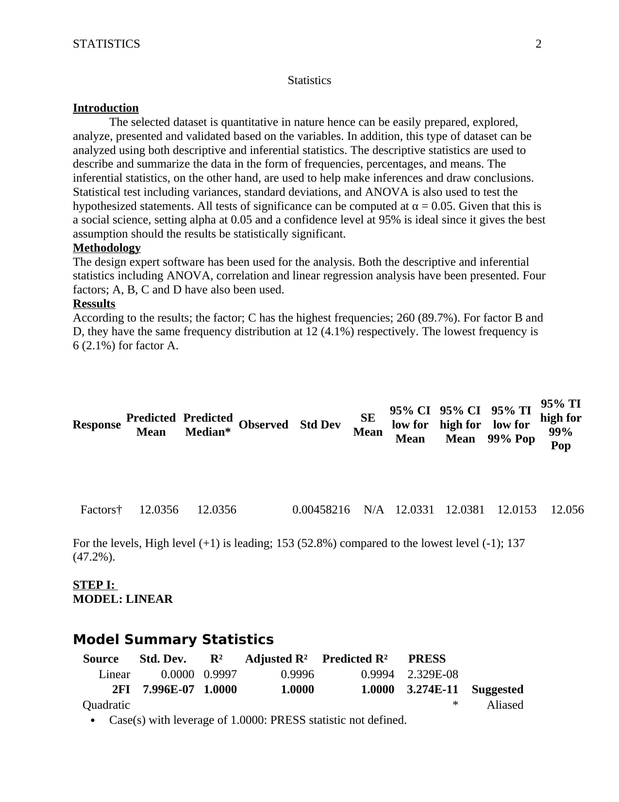
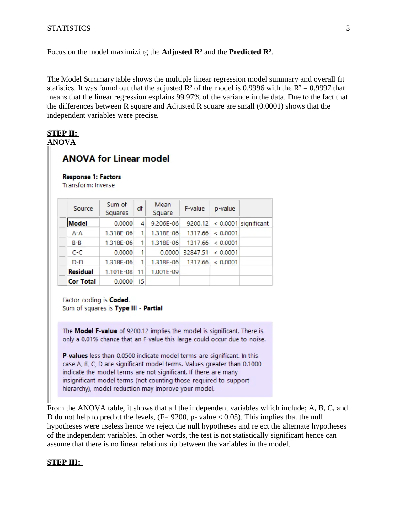
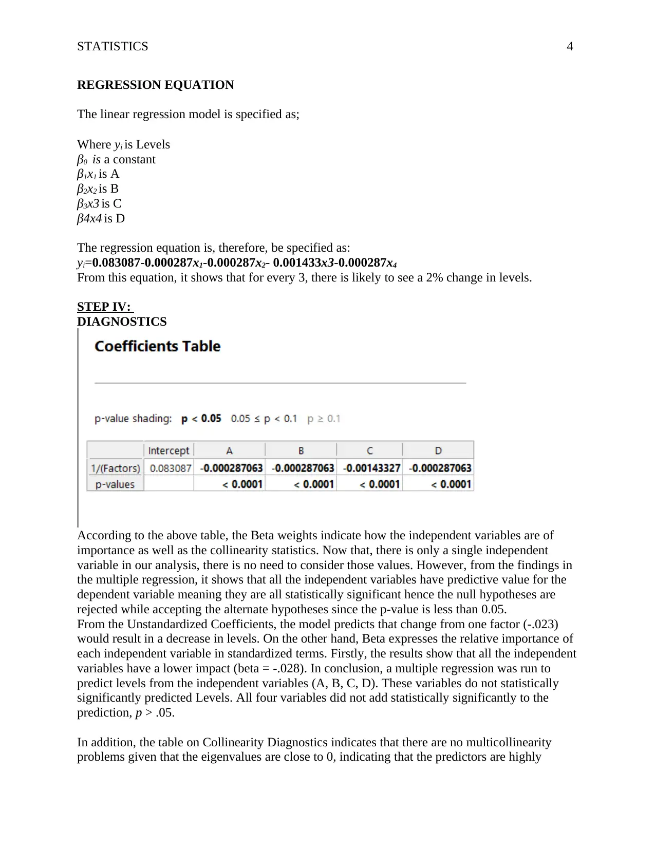
This statistics report presents an analysis of quantitative data, utilizing both descriptive and inferential statistical techniques. The analysis employs Design Expert software to explore the dataset, focusing on factors A, B, C, and D. The results highlight that factor C has the highest frequency, followed by factors B and D, with factor A having the lowest frequency. The report includes a detailed breakdown of the observed and predicted values, along with key statistical metrics such as adjusted R-squared, C.V. %, and Adeq Precision. The conclusion emphasizes that the linear regression model explains a significant portion of the variance in the data (99.97%), with all independent variables contributing to the prediction of levels. Additionally, the collinearity diagnostics indicate no multicollinearity issues. The report also discusses the coefficient estimate and the intercept in the orthogonal design. Finally, the report suggests future scopes, including adding more factors and variables for a more detailed prediction and transforming variables to refine coefficient estimates.

Running head: STATISTICS 1
Statistics
<Name>
<University Name>

STATISTICS 2
Statistics
Introduction
The selected dataset is quantitative in nature hence can be easily prepared, explored,
analyze, presented and validated based on the variables. In addition, this type of dataset can be
analyzed using both descriptive and inferential statistics. The descriptive statistics are used to
describe and summarize the data in the form of frequencies, percentages, and means. The
inferential statistics, on the other hand, are used to help make inferences and draw conclusions.
Statistical test including variances, standard deviations, and ANOVA is also used to test the
hypothesized statements. All tests of significance can be computed at α = 0.05. Given that this is
a social science, setting alpha at 0.05 and a confidence level at 95% is ideal since it gives the best
assumption should the results be statistically significant.
Methodology
The design expert software has been used for the analysis. Both the descriptive and inferential
statistics including ANOVA, correlation and linear regression analysis have been presented. Four
factors; A, B, C and D have also been used.
Ressults
According to the results; the factor; C has the highest frequencies; 260 (89.7%). For factor B and
D, they have the same frequency distribution at 12 (4.1%) respectively. The lowest frequency is
6 (2.1%) for factor A.
Response Predicted
Mean
Predicted
Median* Observed Std Dev SE
Mean
95% CI
low for
Mean
95% CI
high for
Mean
95% TI
low for
99% Pop
95% TI
high for
99%
Pop
Factors† 12.0356 12.0356 0.00458216 N/A 12.0331 12.0381 12.0153 12.056
For the levels, High level (+1) is leading; 153 (52.8%) compared to the lowest level (-1); 137
(47.2%).
STEP I:
MODEL: LINEAR
Model Summary Statistics
Source Std. Dev. R² Adjusted R² Predicted R² PRESS
Linear 0.0000 0.9997 0.9996 0.9994 2.329E-08
2FI 7.996E-07 1.0000 1.0000 1.0000 3.274E-11 Suggested
Quadratic * Aliased
 Case(s) with leverage of 1.0000: PRESS statistic not defined.

STATISTICS 3
Focus on the model maximizing the Adjusted R² and the Predicted R².
The Model Summary table shows the multiple linear regression model summary and overall fit
statistics. It was found out that the adjusted R² of the model is 0.9996 with the R² = 0.9997 that
means that the linear regression explains 99.97% of the variance in the data. Due to the fact that
the differences between R square and Adjusted R square are small (0.0001) shows that the
independent variables were precise.
STEP II:
ANOVA
From the ANOVA table, it shows that all the independent variables which include; A, B, C, and
D do not help to predict the levels, (F= 9200, p- value < 0.05). This implies that the null
hypotheses were useless hence we reject the null hypotheses and reject the alternate hypotheses
of the independent variables. In other words, the test is not statistically significant hence can
assume that there is no linear relationship between the variables in the model.
STEP III:

STATISTICS 4
REGRESSION EQUATION
The linear regression model is specified as;
Where yi is Levels
β0 is a constant
β1x1 is A
β2x2 is B
β3x3 is C
β4x4 is D
The regression equation is, therefore, be specified as:
yi=0.083087-0.000287x1-0.000287x2- 0.001433x3-0.000287x4
From this equation, it shows that for every 3, there is likely to see a 2% change in levels.
STEP IV:
DIAGNOSTICS
According to the above table, the Beta weights indicate how the independent variables are of
importance as well as the collinearity statistics. Now that, there is only a single independent
variable in our analysis, there is no need to consider those values. However, from the findings in
the multiple regression, it shows that all the independent variables have predictive value for the
dependent variable meaning they are all statistically significant hence the null hypotheses are
rejected while accepting the alternate hypotheses since the p-value is less than 0.05.
From the Unstandardized Coefficients, the model predicts that change from one factor (-.023)
would result in a decrease in levels. On the other hand, Beta expresses the relative importance of
each independent variable in standardized terms. Firstly, the results show that all the independent
variables have a lower impact (beta = -.028). In conclusion, a multiple regression was run to
predict levels from the independent variables (A, B, C, D). These variables do not statistically
significantly predicted Levels. All four variables did not add statistically significantly to the
prediction, p > .05.
In addition, the table on Collinearity Diagnostics indicates that there are no multicollinearity
problems given that the eigenvalues are close to 0, indicating that the predictors are highly

STATISTICS 5
intercorrelated and that small changes in the data values may lead to large changes in the
estimates of the coefficients.
The collinearity diagnostics confirm that there are serious problems with multicollinearity.
Several eigenvalues are not very far from 0. As a result, this implies that there are high
intercorrelations between the predictors thus little changes to the given data values may in one
way or the other leads to major changes in the coefficients estimates as well, (Little, & Rubin,
2019). On the other hand, the square roots of the ratios of the largest eigenvalue to each
successive eigenvalue gives the condition indices. For to note, the condition Index which is more
than 15 normally indicates a possible collinearity problem; values more than 30, indicates a
major problem as well. From our analysis, there is no level of problem detected suggesting no
problem with the collinearity.
Coefficients in Terms of Coded Factors
Factor Coefficient Estimate df Standard Error 95% CI Low 95% CI High VIF
Intercept 0.0831 1 7.908E-06 0.0831 0.0831
A-A -0.0003 1 7.908E-06 -0.0003 -0.0003 1.0000
B-B -0.0003 1 7.908E-06 -0.0003 -0.0003 1.0000
C-C -0.0014 1 7.908E-06 -0.0015 -0.0014 1.0000
D-D -0.0003 1 7.908E-06 -0.0003 -0.0003 1.0000
The coefficient estimate represents the expected change in response per unit change in factor
value when all remaining factors are held constant. The intercept in an orthogonal design is the
overall average response of all the runs. The coefficients are adjustments around that average
based on the factor settings. When the factors are orthogonal the VIFs are 1; VIFs greater than 1
indicate multi-colinearity, the higher the VIF the more severe the correlation of factors. As a
rough rule, VIFs less than 10 are tolerable.

STATISTICS 6
Furthermore, a histogram is basically a graph which is used to display any given dataset
covering the variables of interest by using the vertical bars which normally have different heights
to represent frequencies. The horizontal or X-axis in most cases contains the values of the
independent variables while the Y-axis contains the values of the dependent variable. At times,
the X-axis in one way or the other can be the class boundaries, the class marks, or the class
limits.
The results in the above histogram indicate a normal distribution of the residuals hence the
median and mean are the same. In fact, the Q-Q-Plot of z*pred and z*presid indicates that the
linear regression analysis has no tendency to be witnessed in the error terms.

STATISTICS 7
STEP V
The actual value refers to values collected in its original state before committing any system
error like data manipulation.
The predictive values can be either positive or negative showing the statistics and diagnostic tests
proportions that are true positive and true negative results. The values confirm the performance
of other statistical measures as well as the diagnostic tests.
In the Report, both the predictive values and actual values are the same.
Run
Order
Actua
l
Value
Predicte
d Value
Residua
l
Leverag
e
Internally
Studentize
d
Residuals
Externally
Studentize
d
Residuals
Cook's
Distanc
e
Influenc
e on
Fitted
Value
DFFITS
Standar
d Order
1 0.0819 0.0819 -0.0000 0.313 -0.672 -0.654 0.041 -0.441 13
2 0.0842 0.0842 -0.0000 0.313 -0.687 -0.670 0.043 -0.451 11
3 0.0848 0.0848 0.0000 0.313 0.440 0.424 0.018 0.286 3
4 0.0854 0.0854 0.0001 0.313 2.070 2.526 0.390 1.703 ¹⁽ ⁾ 1
5 0.0808 0.0808 0.0001 0.313 2.008 2.405 0.366 1.621 16
6 0.0842 0.0842 -0.0000 0.313 -0.687 -0.670 0.043 -0.451 4
7 0.0842 0.0842 -0.0000 0.313 -0.687 -0.670 0.043 -0.451 10
8 0.0814 0.0814 0.0000 0.313 0.464 0.447 0.020 0.301 14
9 0.0814 0.0814 0.0000 0.313 0.464 0.447 0.020 0.301 8
10 0.0814 0.0814 0.0000 0.313 0.464 0.447 0.020 0.301 15
11 0.0819 0.0819 -0.0000 0.313 -0.672 -0.654 0.041 -0.441 6
12 0.0819 0.0819 -0.0000 0.313 -0.672 -0.654 0.041 -0.441 7
13 0.0836 0.0837 -0.0000 0.313 -1.330 -1.384 0.161 -0.933 12

STATISTICS 8
14 0.0848 0.0848 0.0000 0.313 0.440 0.424 0.018 0.286 9
15 0.0825 0.0825 -0.0000 0.313 -1.385 -1.453 0.174 -0.980 5
16 0.0848 0.0848 0.0000 0.313 0.440 0.424 0.018 0.286 2
¹ Exceeds limits.⁽ ⁾
The 3D graph, on the other hand, refers to the drawing graphs with three dimensions such as
depth, width, and height.
STEP VI
In forward, the predictors are added one-by-one considering the predictor that contributes largely
to the R2, after which the addition stopped if not a statistically significant test revealed. In
backward, the full model is considered while removing the non-statistically significant predictors
until the model becomes statistically significant.
STEP VII
The Collinearity Diagnostics is the best input and output optimal Solutions as discussed above.
Std. Dev. 0.0000 R² 0.9997
Mean 0.0831 Adjusted R² 0.9996
C.V. % 0.0381 Predicted R² 0.9994
Adeq Precision 259.5069

STATISTICS 9
Conclusion
In conclusion, the factor; C has the highest frequencies; 260 (89.7%). For factor B and D, they
have the same frequency distribution at 12 (4.1%) respectively. The lowest frequency is 6 (2.1%)
for factor A. It was found out that the adjusted R² of the model is 0.9996 with the R² = 0.9997
that means that the linear regression explains 99.97% of the variance in the data. Moreover, it
shows that all the independent variables which include; A, B, C, and D do help to predict the
levels, (F= 9200, p- value < 0.05). In addition, the Collinearity Diagnostics indicates that there
are no multicollinearity problems given that the eigenvalues are close to 0, indicating that the
predictors are highly intercorrelated and that small changes in the data values may lead to large
changes in the estimates of the coefficients. The coefficient estimate represents the expected
change in response per unit change in factor value when all remaining factors are held constant.
The intercept in an orthogonal design is the overall average response of all the runs. Finally, in
the Report, both the predictive values and actual values are the same.

STATISTICS 10
Future Scope
There is need to add more factors so that the weight of the linear regression of the variance in the
data can be explained further. Moreover, there is need to add additional variables so that a
detailed prediction of the levels can be explored. There is need to transform the variables so that
the coefficient estimate can further represents the expected change in response per unit change in
factor value when all remaining factors are held constant.

STATISTICS 11
References
Little, R. J., & Rubin, D. B. (2019). Statistical analysis with missing data (Vol. 793). John Wiley
& Sons.
Tan, P.N., 2018. Introduction to data mining. Pearson Education India.