Quantitative Data Analysis Report: BMI at Ages 7 and 50

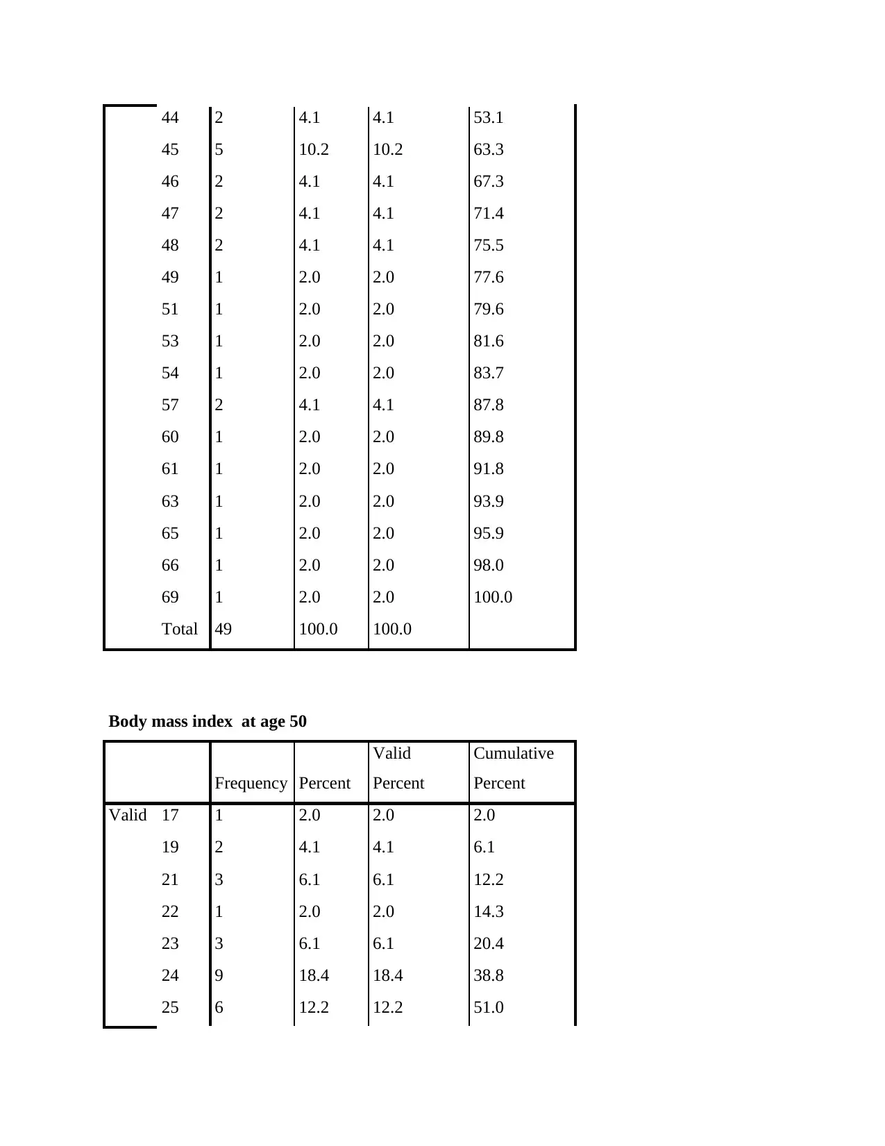
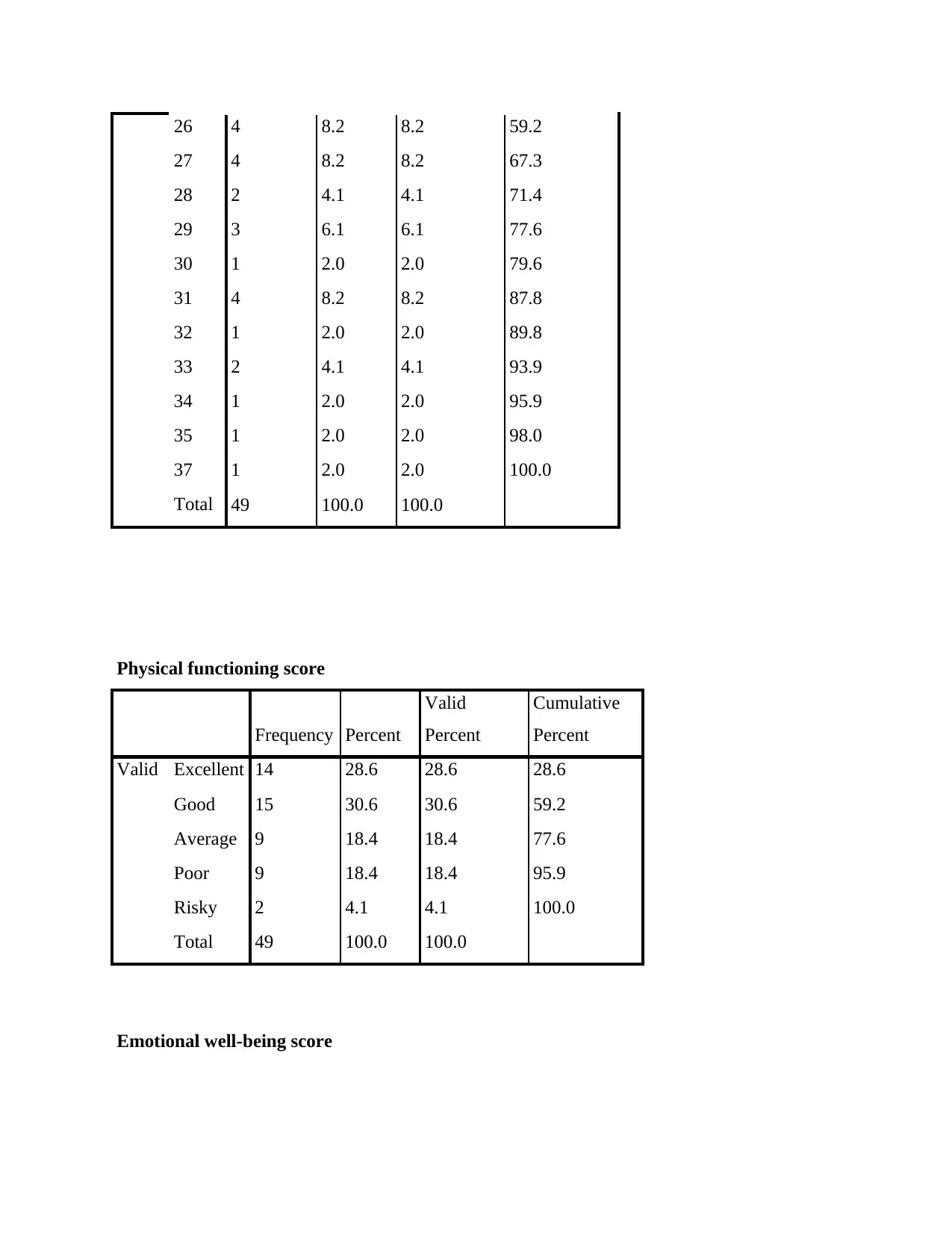
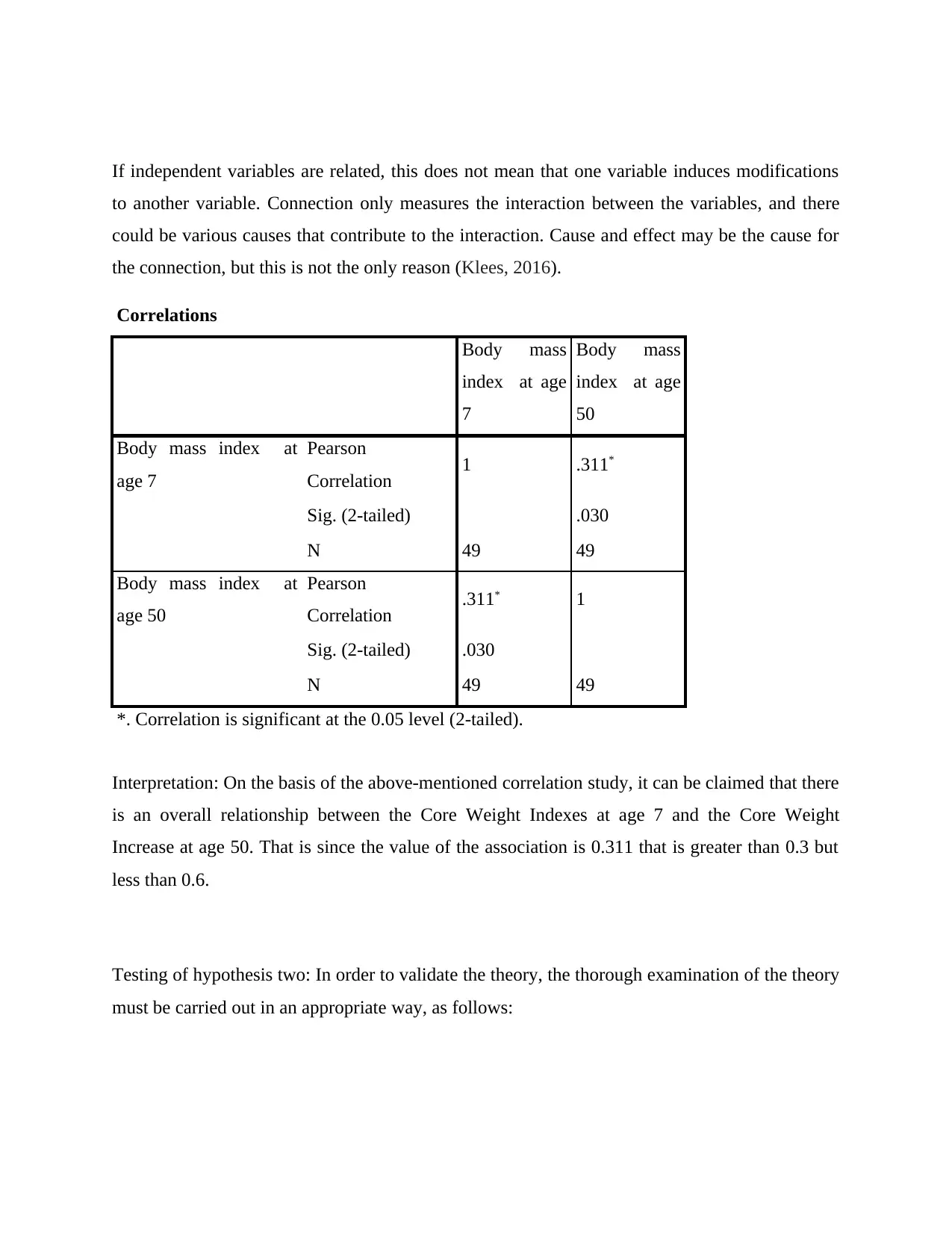
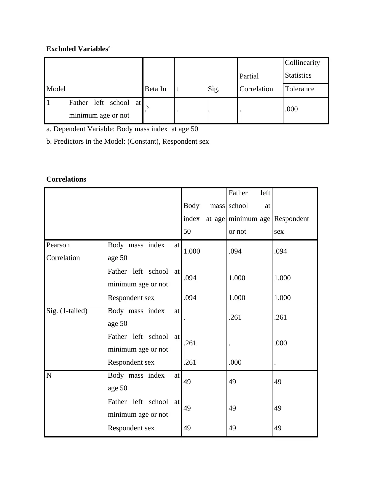
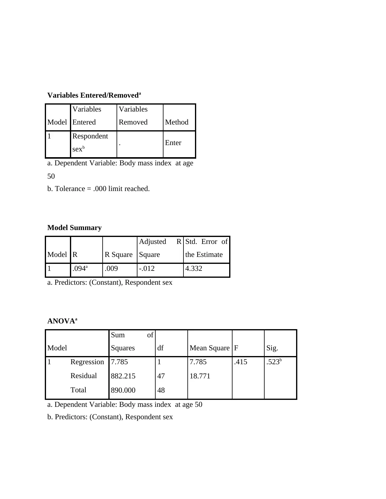
This report presents a quantitative data analysis of BMI, based on data from the National Child Growth Study. The analysis investigates the correlation between BMI at ages 7 and 50, employing SPSS measures to test hypotheses related to BMI and its association with factors such as education and gender. The methodology includes preliminary statistical analysis, correlation analysis, and regression analysis to determine the relationships between variables. The report includes descriptive statistics, correlation matrices, and regression outputs to assess the significance of relationships between variables. The findings indicate a positive correlation between BMI at ages 7 and 50, and the report concludes that there is no significant association between BMI and the gender of the participants. Further analysis is conducted to examine the relationship between BMI at age 7 and well-being variables. The report provides a comprehensive overview of the statistical methods used and the interpretations of the results.

Quantitative Data Analysis Report

Contents
INTRODUCTION.......................................................................................................................................3
I HYPOTHESIS AND METHODOLOGY.................................................................................................3
II. PRELIMINARY STATISTICAL ANALYSIS.......................................................................................3
III. REGRESSION ANALYSIS & INTERPRETATION............................................................................9
CONCLUSION.........................................................................................................................................23
REFERENCES..........................................................................................................................................25

INTRODUCTION
The study is based on an interpretation of the data gathered by the National Child Growth Study,
which monitors a sample of people born in a single week in 1958, at 3-5 years increments
(Ranganathan, Pramesh, & Aggarwal,2017). In order to better evaluate these factors, a number of
SPSS measures have been used to determine if there is an acceptable interaction between the
factors or if there's some important result that can be obtained from a data collection of 50 men
and women.
I HYPOTHESIS AND METHODOLOGY
Qualitative statistics and multiple linear regressions would be tested for correlation among BMI
at 7 and 50 years. Algorithms are trained separately even without a factor answer. Findings shall
be registered and viewed both orally and where applicable, socially. They might have tested
three assumptions:
H1: There is significant relation between Body mass index at age of 7 and at age of 50.
H0: There is no significant relation between Body mass index at age of 7 and at age of 50.
H1: The adiposity at age 50 is measured as body mass index (BMI), is associated with own
education, father’s education and sex.
H0: The adiposity at age 50 is not measured as body mass index (BMI), is associated with own
education, father’s education and sex
II. PRELIMINARY STATISTICAL ANALYSIS
Statistics

Respond
ent sex
Father
left
school
at
minimu
m age
or not
Numb
er of
O-
levels
passed
by
1974
Body
mass
index
at
age 7
Body
mass
index
at
age
50
Physical
functioni
ng score
Emotio
nal
well-
being
score
Social
functioni
ng score
Gener
al
health
score
N Valid 49 49 49 49 49 49 49 49 49
Missi
ng 0 0 0 0 0 0 0 0 0
Mean 1.45 1.45 1.45 45.5
5
26.2
9 2.39 2.41 2.47 2.41
Median 1.00 1.00 1.00 44.0
0
25.0
0 2.00 2.00 2.00 2.00
Std. Deviation .503 .503 .503 9.01
9
4.30
6 1.204 1.098 1.260 1.189
Variance .253 .253 .253 81.3
36
18.5
42 1.451 1.205 1.588 1.413
Respondent sex
Frequency Percent
Valid
Percent
Cumulative
Percent
Valid Male 27 55.1 55.1 55.1
Female 22 44.9 44.9 100.0
Total 49 100.0 100.0
Father left school at minimum age or not

Frequency Percent
Valid
Percent
Cumulative
Percent
Valid yes 27 55.1 55.1 55.1
No 22 44.9 44.9 100.0
Total 49 100.0 100.0
Number of O-levels passed by 1974
Frequency Percent
Valid
Percent
Cumulative
Percent
Valid Yes 27 55.1 55.1 55.1
No 22 44.9 44.9 100.0
Total 49 100.0 100.0
Body mass index at age 7
Frequency Percent
Valid
Percent
Cumulative
Percent
Valid 30 1 2.0 2.0 2.0
34 2 4.1 4.1 6.1
35 1 2.0 2.0 8.2
36 2 4.1 4.1 12.2
37 2 4.1 4.1 16.3
38 2 4.1 4.1 20.4
39 2 4.1 4.1 24.5
40 3 6.1 6.1 30.6
41 2 4.1 4.1 34.7
42 4 8.2 8.2 42.9
43 3 6.1 6.1 49.0

44 2 4.1 4.1 53.1
45 5 10.2 10.2 63.3
46 2 4.1 4.1 67.3
47 2 4.1 4.1 71.4
48 2 4.1 4.1 75.5
49 1 2.0 2.0 77.6
51 1 2.0 2.0 79.6
53 1 2.0 2.0 81.6
54 1 2.0 2.0 83.7
57 2 4.1 4.1 87.8
60 1 2.0 2.0 89.8
61 1 2.0 2.0 91.8
63 1 2.0 2.0 93.9
65 1 2.0 2.0 95.9
66 1 2.0 2.0 98.0
69 1 2.0 2.0 100.0
Total 49 100.0 100.0
Body mass index at age 50
Frequency Percent
Valid
Percent
Cumulative
Percent
Valid 17 1 2.0 2.0 2.0
19 2 4.1 4.1 6.1
21 3 6.1 6.1 12.2
22 1 2.0 2.0 14.3
23 3 6.1 6.1 20.4
24 9 18.4 18.4 38.8
25 6 12.2 12.2 51.0

26 4 8.2 8.2 59.2
27 4 8.2 8.2 67.3
28 2 4.1 4.1 71.4
29 3 6.1 6.1 77.6
30 1 2.0 2.0 79.6
31 4 8.2 8.2 87.8
32 1 2.0 2.0 89.8
33 2 4.1 4.1 93.9
34 1 2.0 2.0 95.9
35 1 2.0 2.0 98.0
37 1 2.0 2.0 100.0
Total 49 100.0 100.0
Physical functioning score
Frequency Percent
Valid
Percent
Cumulative
Percent
Valid Excellent 14 28.6 28.6 28.6
Good 15 30.6 30.6 59.2
Average 9 18.4 18.4 77.6
Poor 9 18.4 18.4 95.9
Risky 2 4.1 4.1 100.0
Total 49 100.0 100.0
Emotional well-being score

Frequency Percent
Valid
Percent
Cumulative
Percent
Valid excellent 11 22.4 22.4 22.4
good 18 36.7 36.7 59.2
avergae 10 20.4 20.4 79.6
poor 9 18.4 18.4 98.0
risky 1 2.0 2.0 100.0
Total 49 100.0 100.0
Social functioning score
Frequency Percent
Valid
Percent
Cumulative
Percent
Valid excellent 13 26.5 26.5 26.5
good 16 32.7 32.7 59.2
avergae 7 14.3 14.3 73.5
poor 10 20.4 20.4 93.9
risky 3 6.1 6.1 100.0
Total 49 100.0 100.0
General health score
Frequency Percent
Valid
Percent
Cumulative
Percent
Valid excellent 12 24.5 24.5 24.5
good 19 38.8 38.8 63.3
avergae 6 12.2 12.2 75.5

poor 10 20.4 20.4 95.9
risky 2 4.1 4.1 100.0
Total 49 100.0 100.0
Analysis- The tables above showed that the overall and standardized deviations of each factor are
not similar to one another. As a consequence, it can be claimed that there is no connection
between the data collection of sample participants. Apart from this, the average weight masses
indexes level at aged 7 is greater than the mean weight masses level at age 50. This indicates that
even at the age of seven learners around the world was much improved there was a good
difference among age and length.
III. REGRESSION ANALYSIS & INTERPRETATION
Testing of hypothesis one: In order to confirm above - the thesis, a number of SPSS experiments
have been carried out in an appropriate manner and is as continues to follow:
H1: There is significant relation between Body mass index at age of 7 and at age of 50.
H0: There is no significant relation between Body mass index at age of 7 and at age of 50.
In order to such hypothesis, correlation analysis is crucial which is performed below in such
manner:
Correlation: Correspondence is a mathematical indicator of the association between two
variables. The test is best used in factors that display a linear connection between the qualities.
The software fit could be visually depicted in a scatter graph (Hayes & Montoya, 2017). Using a
scatter graph, we will usually analyze the correlation between different variables to assess if
they're not associated. Correlation of causal relationships must not be mistaken. The common
phrase "correlation does not equal causation" is key to the interpretation of the two mathematical
principles.

If independent variables are related, this does not mean that one variable induces modifications
to another variable. Connection only measures the interaction between the variables, and there
could be various causes that contribute to the interaction. Cause and effect may be the cause for
the connection, but this is not the only reason (Klees, 2016).
Correlations
Body mass
index at age
7
Body mass
index at age
50
Body mass index at
age 7
Pearson
Correlation 1 .311*
Sig. (2-tailed) .030
N 49 49
Body mass index at
age 50
Pearson
Correlation .311* 1
Sig. (2-tailed) .030
N 49 49
*. Correlation is significant at the 0.05 level (2-tailed).
Interpretation: On the basis of the above-mentioned correlation study, it can be claimed that there
is an overall relationship between the Core Weight Indexes at age 7 and the Core Weight
Increase at age 50. That is since the value of the association is 0.311 that is greater than 0.3 but
less than 0.6.
Testing of hypothesis two: In order to validate the theory, the thorough examination of the theory
must be carried out in an appropriate way, as follows:

Excluded Variablesa
Model Beta In t Sig.
Partial
Correlation
Collinearity
Statistics
Tolerance
1 Father left school at
minimum age or not .b . . . .000
a. Dependent Variable: Body mass index at age 50
b. Predictors in the Model: (Constant), Respondent sex
Correlations
Body mass
index at age
50
Father left
school at
minimum age
or not
Respondent
sex
Pearson
Correlation
Body mass index at
age 50 1.000 .094 .094
Father left school at
minimum age or not .094 1.000 1.000
Respondent sex .094 1.000 1.000
Sig. (1-tailed) Body mass index at
age 50 . .261 .261
Father left school at
minimum age or not .261 . .000
Respondent sex .261 .000 .
N Body mass index at
age 50 49 49 49
Father left school at
minimum age or not 49 49 49
Respondent sex 49 49 49

Variables Entered/Removeda
Model
Variables
Entered
Variables
Removed Method
1 Respondent
sexb . Enter
a. Dependent Variable: Body mass index at age
50
b. Tolerance = .000 limit reached.
Model Summary
Model R R Square
Adjusted R
Square
Std. Error of
the Estimate
1 .094a .009 -.012 4.332
a. Predictors: (Constant), Respondent sex
ANOVAa
Model
Sum of
Squares df Mean Square F Sig.
1 Regression 7.785 1 7.785 .415 .523b
Residual 882.215 47 18.771
Total 890.000 48
a. Dependent Variable: Body mass index at age 50
b. Predictors: (Constant), Respondent sex

Coefficientsa
Model
Unstandardized
Coefficients
Standardized
Coefficients
t Sig.B Std. Error Beta
1 (Constant) 25.125 1.906 13.180 .000
Respondent sex .801 1.244 .094 .644 .523
a. Dependent Variable: Body mass index at age 50
Excluded Variablesa
Model Beta In t Sig.
Partial
Correlation
Collinearity
Statistics
Tolerance
1 Father left school at
minimum age or not .b . . . .000
a. Dependent Variable: Body mass index at age 50
b. Predictors in the Model: (Constant), Respondent sex
Collinearity Diagnosticsa
Model Dimension Eigenvalue
Condition
Index
Variance Proportions
(Constant)
Respondent
sex
1 1 1.946 1.000 .03 .03
2 .054 5.993 .97 .97
a. Dependent Variable: Body mass index at age 50
Interpretation: In the grounds of the above-mentioned correlation analysis, it can be calculated
whether the significance of the meaningful gap is 0.523, which is more than 0.05. This indicates
that there is no important association between the bmi and the gender of the participants. That's

because of the uneven interaction between the two variables (Austin & Merlo, 2017). With the
exception of this, it can be confirmed from Pearson's association that there really is no
association among different types of variables, such as the bmi only at age of 50 as well as the
gender and literacy for participants. It has become achieved in line with the value of the
comparison below 3.
Regression on body mass index at age of 7 and wellbeing variables:
Descriptive Statistics
Mean
Std.
Deviation N
Body mass index at
age 7 45.55 9.019 49
Physical functioning
score 2.39 1.204 49
Emotional well-being
score 2.41 1.098 49
Social functioning
score 2.47 1.260 49
General health score 2.41 1.189 49
Correlations
Body
mass
index at
age 7
Physical
functioning
score
Emotional
well-being
score
Social
functioning
score
General
health
score
Pearson
Correlation
Body mass
index at age
7
1.000 .099 -.246 -.073 -.031

Physical
functioning
score
.099 1.000 .035 -.191 .135
Emotional
well-being
score
-.246 .035 1.000 -.141 .285
Social
functioning
score
-.073 -.191 -.141 1.000 -.339
General
health score -.031 .135 .285 -.339 1.000
Sig. (1-
tailed)
Body mass
index at age
7
. .250 .044 .310 .416
Physical
functioning
score
.250 . .405 .094 .178
Emotional
well-being
score
.044 .405 . .166 .024
Social
functioning
score
.310 .094 .166 . .009
General
health score .416 .178 .024 .009 .
N Body mass
index at age
7
49 49 49 49 49

Physical
functioning
score
49 49 49 49 49
Emotional
well-being
score
49 49 49 49 49
Social
functioning
score
49 49 49 49 49
General
health score 49 49 49 49 49
Variables Entered/Removeda
Model
Variables
Entered
Variables
Removed Method
1 General
health score,
Physical
functioning
score,
Emotional
well-being
score, Social
functioning
scoreb
. Enter
a. Dependent Variable: Body mass index at age
7
b. All requested variables entered.

Model Summary
Model R
R
Square
Adjusted R
Square
Std. Error of
the Estimate
Change Statistics
R Square
Change
F
Change df1 df2
Sig. F
Change
1 .283a .080 -.003 9.033 .080 .961 4 44 .438
a. Predictors: (Constant), General health score, Physical functioning score, Emotional well-
being score, Social functioning score
ANOVAa
Model
Sum of
Squares df Mean Square F Sig.
1 Regression 313.612 4 78.403 .961 .438b
Residual 3590.510 44 81.603
Total 3904.122 48
a. Dependent Variable: Body mass index at age 7
b. Predictors: (Constant), General health score, Physical functioning score,
Emotional well-being score, Social functioning score
Coefficientsa
Model
Unstandardize
d Coefficients
Standardize
d
Coefficients
t Sig.
Correlations
Collinearity
Statistics
B
Std.
Error Beta
Zero
-
order
Partia
l Part
Toleranc
e VIF

1 (Constant) 50.764 6.009 8.44
8 .000
Physical
functionin
g score
.677 1.106 .090 .612 .544 .099 .092 .088 .958 1.044
Emotional
well-being
score
-2.157 1.241 -.263
-
1.73
9
.089 -.246 -.254 -.25
1 .917 1.091
Social
functionin
g score
-.663 1.115 -.093 -.594 .555 -.073 -.089 -.08
6 .861 1.161
General
health
score
.001 1.209 .000 .001 1.00
0 -.031 .000 .000 .823 1.215
a. Dependent Variable: Body mass index at age 7
Collinearity Diagnosticsa
Mode
l
Dimensio
n
Eigenvalu
e
Conditio
n Index
Variance Proportions
(Constant
)
Physical
functionin
g score
Emotiona
l well-
being
score
Social
functionin
g score
Genera
l health
score
1 1 4.365 1.000 .00 .01 .01 .01 .01
2 .289 3.887 .00 .03 .02 .41 .12
3 .188 4.813 .00 .70 .18 .00 .08
4 .122 5.990 .00 .04 .65 .04 .56
5 .036 11.089 1.00 .22 .14 .54 .23
a. Dependent Variable: Body mass index at age 7

Interpretation: In the grounds of the aforementioned analysis, it can be claimed that this is a
substantial discrepancy among the two, since the P meaning is greater than 0.05, which is 0.438.
Apart of this, on grounds of the correlation, it could be claimed that there is a weak relationship
between parameters since the meaning of and factor is lower than 0.3.
Regression on body mass index at age of 50 and wellbeing variables and respondent sex:
Descriptive Statistics
Mean
Std.
Deviation N
Body mass index at
age 50 26.29 4.306 49
Physical functioning
score 2.39 1.204 49
Emotional well-being
score 2.41 1.098 49
Social functioning
score 2.47 1.260 49
General health score 2.41 1.189 49
Respondent sex 1.45 .503 49
Correlations

Body
mass
index
at age
50
Physical
functioning
score
Emotional
well-being
score
Social
functioning
score
General
health
score
Respondent
sex
Pearson
Correlation
Body mass
index at
age 50
1.000 -.275 -.435 .290 -.040 .094
Physical
functioning
score
-.275 1.000 .035 -.191 .135 -.122
Emotional
well-being
score
-.435 .035 1.000 -.141 .285 .039
Social
functioning
score
.290 -.191 -.141 1.000 -.339 .121
General
health score -.040 .135 .285 -.339 1.000 -.034
Respondent
sex .094 -.122 .039 .121 -.034 1.000
Sig. (1-
tailed)
Body mass
index at
age 50
. .028 .001 .022 .394 .261
Physical
functioning
score
.028 . .405 .094 .178 .203
Emotional
well-being
score
.001 .405 . .166 .024 .396

Social
functioning
score
.022 .094 .166 . .009 .204
General
health score .394 .178 .024 .009 . .408
Respondent
sex .261 .203 .396 .204 .408 .
N Body mass
index at
age 50
49 49 49 49 49 49
Physical
functioning
score
49 49 49 49 49 49
Emotional
well-being
score
49 49 49 49 49 49
Social
functioning
score
49 49 49 49 49 49
General
health score 49 49 49 49 49 49
Respondent
sex 49 49 49 49 49 49
Variables Entered/Removeda
Model
Variables
Entered
Variables
Removed Method

1 Respondent
sex, General
health score,
Physical
functioning
score,
Emotional
well-being
score, Social
functioning
scoreb
. Enter
a. Dependent Variable: Body mass index at age
50
b. All requested variables entered.
Model Summary
Model R
R
Square
Adjusted R
Square
Std. Error of
the Estimate
Change Statistics
R Square
Change
F
Change df1 df2
Sig. F
Change
1 .574a .329 .251 3.726 .329 4.221 5 43 .003
a. Predictors: (Constant), Respondent sex, General health score, Physical functioning score,
Emotional well-being score, Social functioning score
ANOVAa
Model
Sum of
Squares df Mean Square F Sig.
1 Regression 292.990 5 58.598 4.221 .003b
Residual 597.010 43 13.884

Total 890.000 48
a. Dependent Variable: Body mass index at age 50
b. Predictors: (Constant), Respondent sex, General health score, Physical
functioning score, Emotional well-being score, Social functioning score
Interpretation: Based from the above figures, it can be calculated there is a correlation between
Body fat percentage only at age of 50, gender and very well parameters among participants. The
reasoning behind this is that both R and R calculated value is below the standard of estimates
(Sellam & Poovammal, 2016). Apart of this, there is a large gap in the data collection and the
meaning is 0.003, which is lower than 0.05.
CONCLUSION
On the grounds from the above study, it can be inferred there is a typical relationship among
participants who Body fat percentage at the age of 7 and 50 is distinct. This was tested in line
with the SPSS experiments and the correlation. Although this can be said from the first
conceptual framework of the study that perhaps the assumption is false and it has been checked
under logistic regression. Apart from it a multiple regressions is often applied to any other factor
under which a discrete result is generated.

REFERENCES
Schroeder, L. D., Sjoquist, D. L., & Stephan, P. E. (2016). Understanding regression analysis:
An introductory guide (Vol. 57). Sage Publications.
Ranganathan, P., Pramesh, C. S., & Aggarwal, R. (2017). Common pitfalls in statistical analysis:
logistic regression. Perspectives in clinical research, 8(3), 148.
Hayes, A. F., & Montoya, A. K. (2017). A tutorial on testing, visualizing, and probing an
interaction involving a multicategorical variable in linear regression analysis. Communication
Methods and Measures, 11(1), 1-30.
Klees, S. (2016). Inferences from regression analysis: Are they valid. Real World Economics
Review, 74, 85-97.
Austin, P. C., & Merlo, J. (2017). Intermediate and advanced topics in multilevel logistic
regression analysis. Statistics in medicine, 36(20), 3257-3277.
Sellam, V., & Poovammal, E. (2016). Prediction of crop yield using regression analysis. Indian
Journal of Science and Technology, 9(38), 1-5.
Zhang, X., Sun, X., Wang, J., Tang, L., & Xie, A. (2017). Prevalence of rapid eye movement
sleep behavior disorder (RBD) in Parkinson’s disease: a meta and meta-regression
analysis. Neurological Sciences, 38(1), 163-170.