Quantitative Finance and Financial Market Assignment - Course Code XYZ

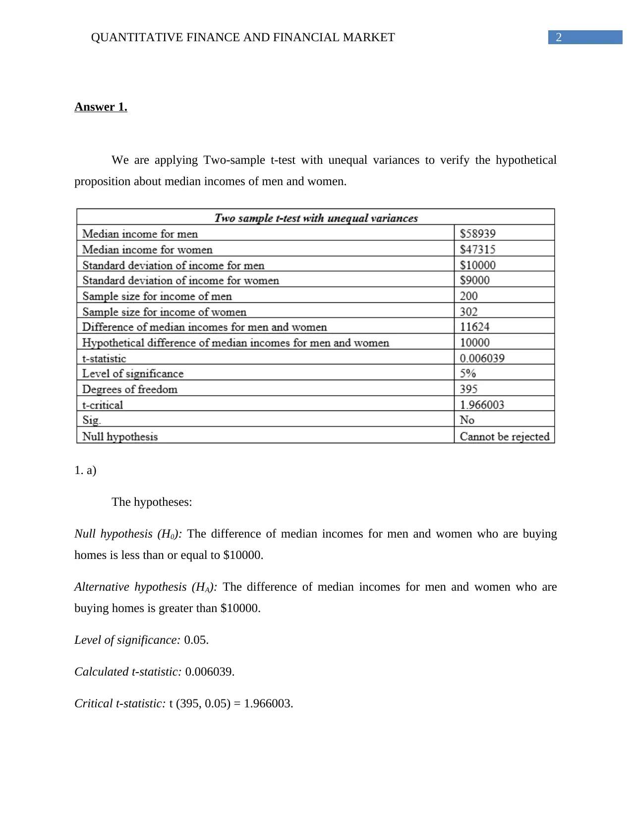
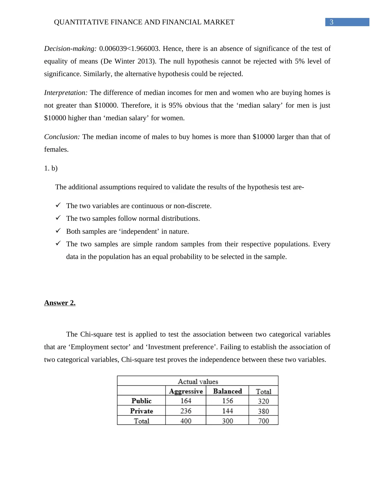
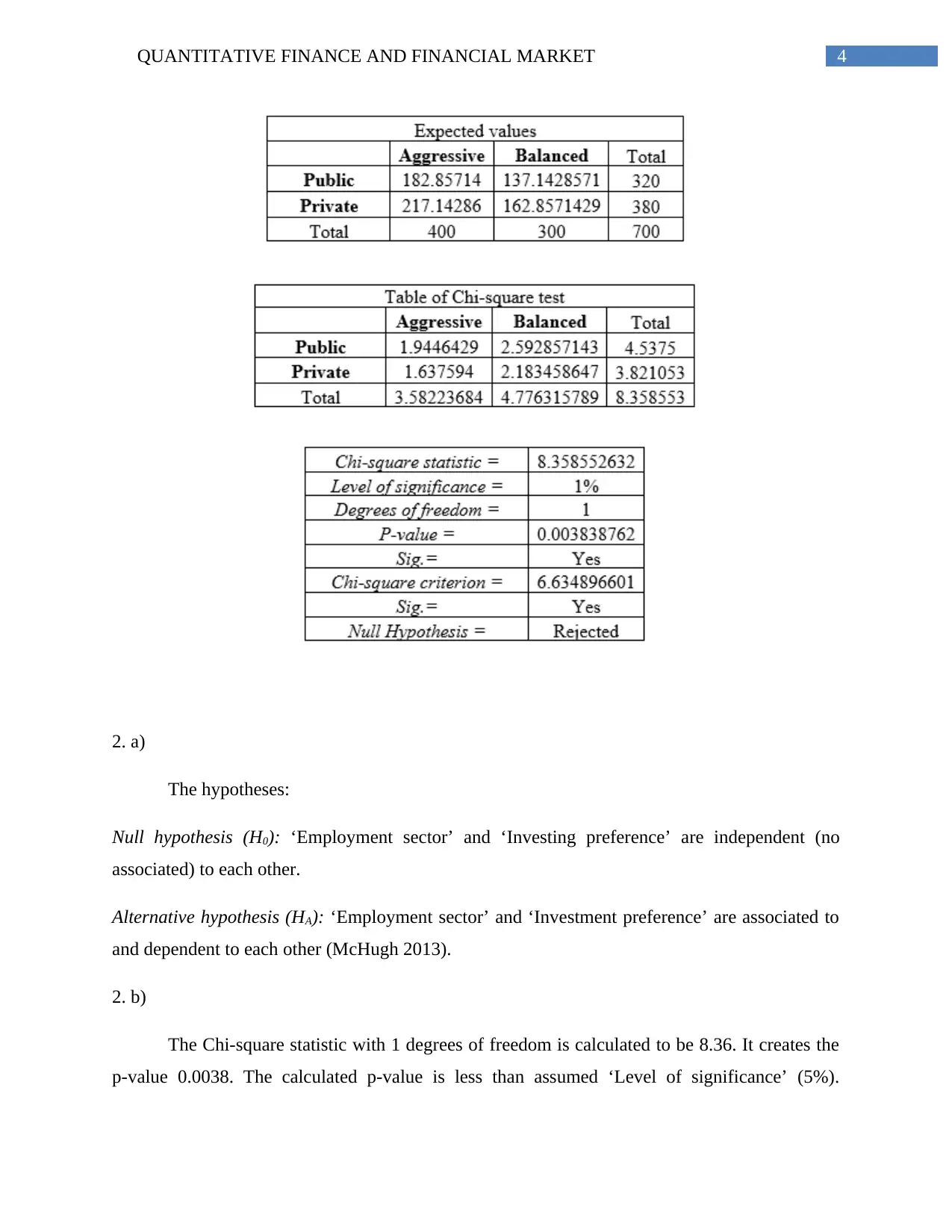
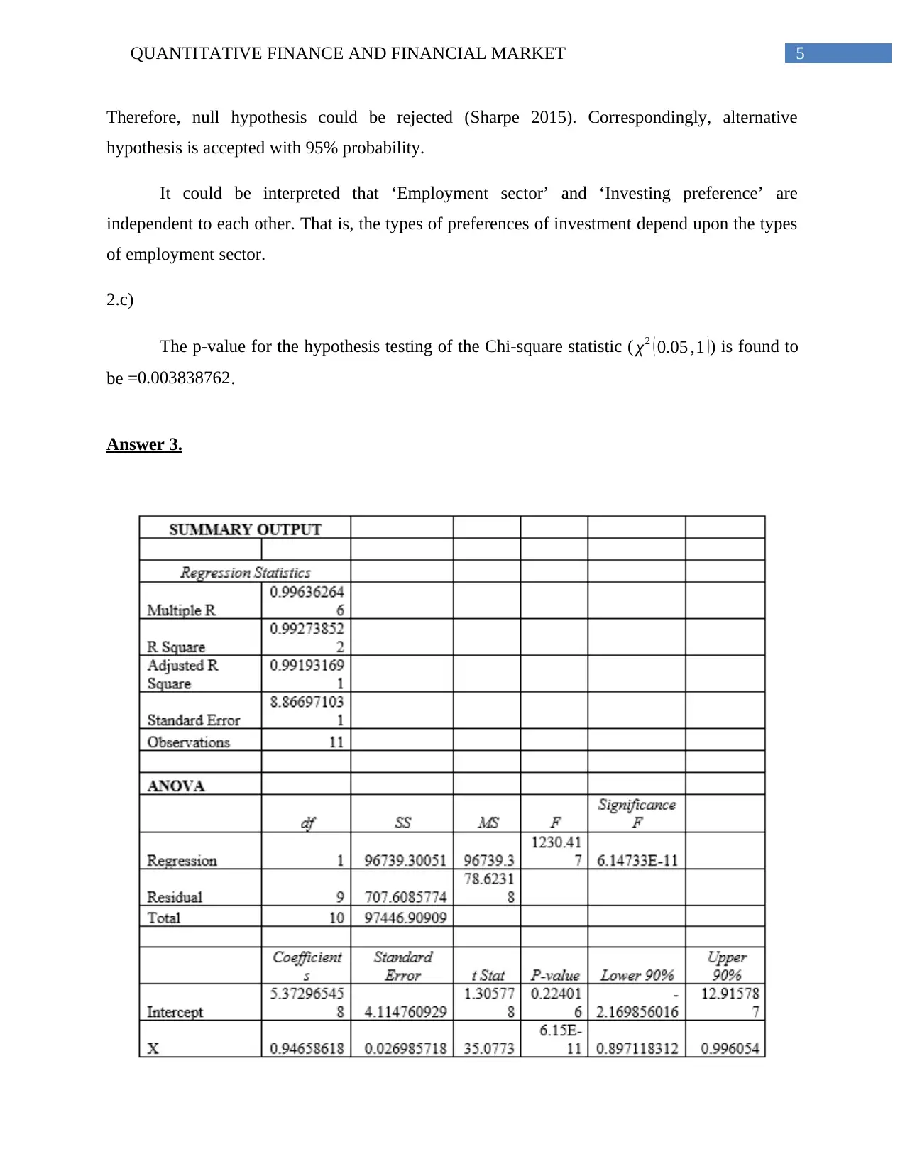
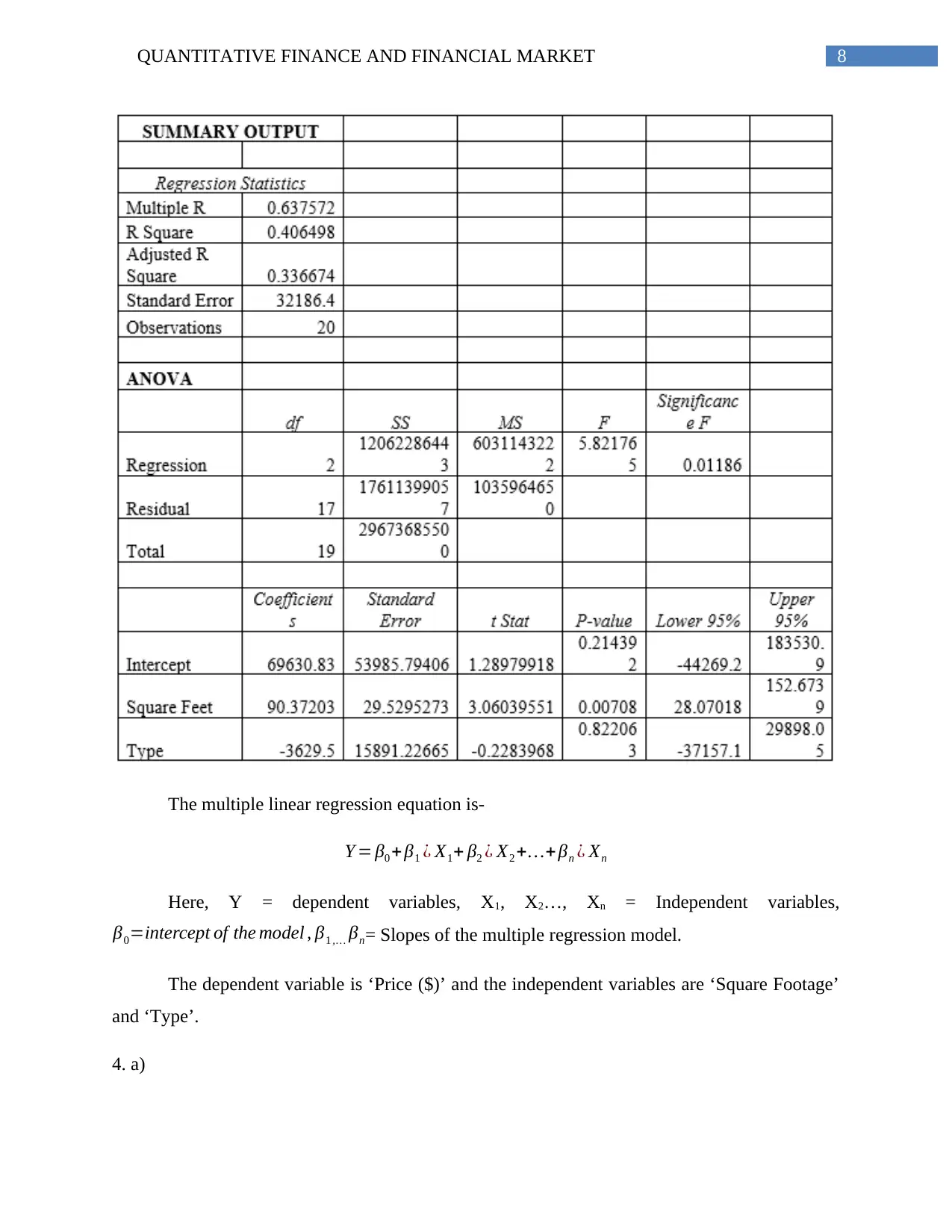
This assignment solution addresses several key concepts in quantitative finance and financial markets. It begins with a two-sample t-test to compare median incomes of men and women, followed by a Chi-square test to analyze the association between employment sector and investment preferences. The solution then delves into regression analysis, including least squares regression to predict account balances and multiple linear regression to predict housing prices based on square footage and type. Furthermore, the assignment includes time series analysis using dummy variables to forecast client generation and concludes with portfolio optimization, calculating expected returns and standard deviations for various stock combinations to construct an efficient frontier. The solution demonstrates the application of statistical methods to real-world financial scenarios, offering insights into market analysis, investment strategies, and risk management.

Running Head: QUANTITATIVE FINANCE AND FINANCIAL MARKET
Quantitative Finance and Financial Market
Name of the student:
Name of the university:
Course ID:

1QUANTITATIVE FINANCE AND FINANCIAL MARKET
Table of Contents
Answer 1..........................................................................................................................................2
Answer 2..........................................................................................................................................3
Answer 3..........................................................................................................................................5
Answer 4..........................................................................................................................................7
Answer 5..........................................................................................................................................9
Answer 6........................................................................................................................................11
Answer 7........................................................................................................................................14
References:....................................................................................................................................19

2QUANTITATIVE FINANCE AND FINANCIAL MARKET
Answer 1.
We are applying Two-sample t-test with unequal variances to verify the hypothetical
proposition about median incomes of men and women.
1. a)
The hypotheses:
Null hypothesis (H0): The difference of median incomes for men and women who are buying
homes is less than or equal to $10000.
Alternative hypothesis (HA): The difference of median incomes for men and women who are
buying homes is greater than $10000.
Level of significance: 0.05.
Calculated t-statistic: 0.006039.
Critical t-statistic: t (395, 0.05) = 1.966003.

3QUANTITATIVE FINANCE AND FINANCIAL MARKET
Decision-making: 0.006039<1.966003. Hence, there is an absence of significance of the test of
equality of means (De Winter 2013). The null hypothesis cannot be rejected with 5% level of
significance. Similarly, the alternative hypothesis could be rejected.
Interpretation: The difference of median incomes for men and women who are buying homes is
not greater than $10000. Therefore, it is 95% obvious that the ‘median salary’ for men is just
$10000 higher than ‘median salary’ for women.
Conclusion: The median income of males to buy homes is more than $10000 larger than that of
females.
1. b)
The additional assumptions required to validate the results of the hypothesis test are-
 The two variables are continuous or non-discrete.
 The two samples follow normal distributions.
 Both samples are ‘independent’ in nature.
 The two samples are simple random samples from their respective populations. Every
data in the population has an equal probability to be selected in the sample.
Answer 2.
The Chi-square test is applied to test the association between two categorical variables
that are ‘Employment sector’ and ‘Investment preference’. Failing to establish the association of
two categorical variables, Chi-square test proves the independence between these two variables.

4QUANTITATIVE FINANCE AND FINANCIAL MARKET
2. a)
The hypotheses:
Null hypothesis (H0): ‘Employment sector’ and ‘Investing preference’ are independent (no
associated) to each other.
Alternative hypothesis (HA): ‘Employment sector’ and ‘Investment preference’ are associated to
and dependent to each other (McHugh 2013).
2. b)
The Chi-square statistic with 1 degrees of freedom is calculated to be 8.36. It creates the
p-value 0.0038. The calculated p-value is less than assumed ‘Level of significance’ (5%).

5QUANTITATIVE FINANCE AND FINANCIAL MARKET
Therefore, null hypothesis could be rejected (Sharpe 2015). Correspondingly, alternative
hypothesis is accepted with 95% probability.
It could be interpreted that ‘Employment sector’ and ‘Investing preference’ are
independent to each other. That is, the types of preferences of investment depend upon the types
of employment sector.
2.c)
The p-value for the hypothesis testing of the Chi-square statistic ( χ2 ( 0.05 ,1 )) is found to
be =0.003838762.
Answer 3.

6QUANTITATIVE FINANCE AND FINANCIAL MARKET
The least square regression equation is-
Y = β0 + β1∗X
Here, Y = dependent variables, X = Independent variable, β0=intercept of the model , β1=
slope of the least square regression model.
The dependent variable (Y) is the actual balance and the independent variable (X) is the
computer-generated account balance in this regression model.
3. a)
The least square regression equation-
‘The actual balance (Y)’ = 5.372965458 + 0.94658618* ‘The computer-generated account
balance (X)’.
3. b)
If the computer-generated account balance (X) was 100, then the actual account balance
as confirmed by the accountant is-
The actual balance (Y) = 5.372965458 + 0.94658618 * 100 = 5.372965458 + 94.658618 =
100.0316.
3.c)
The regression equations of upper and lower 90% confidence limits are-
‘The actual balance (YUpper)’ = 12.915787 + 0.996054 * ‘The computer-generated balance’.
‘The actual balance (YLower)’ = -2.169856016 + 0.897118312 * ‘The computer-generated
balance’.
While the computer-generated balance for Timothy Jones is 100, then
‘The actual balance (YUpper)’ = 12.915787 + 0.996054 * 100 = 12.915787 + 99.6054 = 112.52.

7QUANTITATIVE FINANCE AND FINANCIAL MARKET
‘The actual balance (YLower)’ = -2.169856016 + 0.897118312 * 100 = 87.54.
The 90% interval estimates are = (87.54, 112.52).
3. d)
The average upper and lower 90% confidence limits of predicted actual balance when all
the computer-generated balances are same is given by- (101.81, 128.37).
It means that predicted average actual balance of the investors lies in the interval of
$101.81 to $128.37 with 90% probability.
Answer 4.

8QUANTITATIVE FINANCE AND FINANCIAL MARKET
The multiple linear regression equation is-
Y = β0 + β1 ¿ X1+ β2 ¿ X2 +…+ βn ¿ Xn
Here, Y = dependent variables, X1, X2…, Xn = Independent variables,
β0=intercept of the model , β1 ,… βn= Slopes of the multiple regression model.
The dependent variable is ‘Price ($)’ and the independent variables are ‘Square Footage’
and ‘Type’.
4. a)

9QUANTITATIVE FINANCE AND FINANCIAL MARKET
The regression equation to predict the selling price for residences-
‘Price ($)’ = 69630.83 + 90.37203 * ‘Square Footage’ -3629.5 * ‘Type’ (Montgomery, Peck and
Vining 2012)
4. b)
The first slope parameter (β1) (90.3703) is positive. It interprets that the independent
variable ‘Square Footage’ has positive association with the dependent variable ‘Price ($)’.
Therefore, for higher sizes of real estate in terms of square footage, the price also gets higher.
The second slope parameter (β2) (-3629.5) is negative. In this case, the independent
variable is a binary variable with two levels 0 and 1. ‘1’ is ‘condominium’ and ‘0’ is a ‘single-
family home’. The negative value of slope refers that for higher value (1=condominium) of the
predictor ‘Type’, the dependent variable ‘Price ($)’ decreases. Similarly, for lower value
(0=single-family home) of the predictor ‘Type’, the dependent variable ‘Price ($)’ increases.
In summary, β1 and β2 show that for greater square footage and single-family home, the
price of the real-estate enhances.
4. c)
The regression equation that describes the relationship between selling price and square
footage of
 ‘Condominiums’-
‘Price ($)’ = 69630.83 + 90.37203 * ‘Square Footage’ -3629.5 * 1
= (69630.83 – 3629.5) + 90.37203* ‘Square Footage’
= 66001.33 + 90.37203 * ‘Square Footage’
 ‘Single-family home’-
‘Price ($)’ = 69630.83 + 90.37203 * ‘Square Footage’ -3629.5 * 0
= 69630.83 + 90.37203 * ‘Square Footage’

10QUANTITATIVE FINANCE AND FINANCIAL MARKET
4. d)
The F-statistic indicates the relation between two slope values (β1 and β2). The F-statistic
is 5.821765 with p-value 0.01186. The p-value is less than 0.05. Therefore, it could be stated that
slopes of selling-price (β0), slopes of types of real-estate (condominium and single-family home)
(β1) and square footage (β2) are unrelated to each other (Ngo and La Puente 2012). Hence,
selling-price and the square footage are different between ‘condominiums’ and ‘single-family
homes’.
Answer 5.
5. a)
The graph depicts the trend of number of new clients generated for four quarters for four
years. Overall, the numbers of new clients generated is highest in third quarters of chosen years
and lowest in second quarters of these years. Overall, the highest clients are generated in 2007

11QUANTITATIVE FINANCE AND FINANCIAL MARKET
and lowest in 2006. Individually, most of the new clients are generated in 3rd quarter of 2007 and
least clients are generated in 1st quarter of 2006.
Therefore, it could be said that the number of new clients generated increases after 1st
quarter of the year and then again decreases in 3rd and 4th quarter.
5. b)
The first quarter is denoted by the dummy variable (S1 =1, S2 = 0, S3 =0), the second
quarter is denoted by the dummy variable (S1 =0, S2 =1, S3=0), the third quarter is denoted by
the dummy variable (S1 =0, S2 = 0, S3 =1) and the fourth quarter is denoted by the dummy
variable (S1 =0, S2 =0, S3 =0). The transformation is essential for multiple regression equation.