Quantitative Finance: Statistical Analysis, CI, and Portfolio Report

This report presents a comprehensive analysis of quantitative finance, focusing on the application of statistical tools in financial markets. The research includes regression analysis, confidence interval calculations, and correlation analysis to identify relationships between variables. The report also addresses data quality and the selection of appropriate statistical tools. Furthermore, it explores portfolio return and standard deviation, identifying portfolios with optimal risk-return profiles. The study covers various aspects of financial data analysis, providing insights into market trends and investment strategies. The report includes tables, charts and graphs to illustrate the analysis and findings. It also includes t-tests and ANOVA tests to identify significant differences between groups and variables. The conclusion summarizes the key findings and their implications for financial decision-making.

QUANTITATIVE FINANCE & FINANCIAL
MARKETS

EXECUTIVE SUMMARY
Present research study is conducted in respect to developing strong knowledge of
statistical tools. In the report, regression analysis and CI calculation is done. It is identified that
data quality is the one of the common point where emphasis must be given so that accurate
results can be obtained. Apart from this, due importance must be given on selection of right tool
for data analysis. Common issues faced in respect to application of statistical methods is also
explained in detail in the report. In this way entire research work is carried out

TABLE OF CONTENTS
INTRODUCTION...........................................................................................................................1
Question 1........................................................................................................................................1
(a)Regression equation................................................................................................................1
(b) Correlation between variables...............................................................................................2
© Most under-priced and overpriced car by residuals................................................................2
Question 2........................................................................................................................................3
(a)Line chart for three sets of data..............................................................................................3
(b) Descriptive statistics..............................................................................................................3
© Interpretation of data...............................................................................................................4
(d) Moving average and charts plotting......................................................................................5
( e) Histogram.............................................................................................................................7
(f) Normal distribution................................................................................................................8
Question 3........................................................................................................................................9
Identification of difference between A and B, B and C..............................................................9
Question 4......................................................................................................................................10
(a)Calculating confidence interval............................................................................................10
(b) Z test....................................................................................................................................11
© Performance of test...............................................................................................................11
Question 5......................................................................................................................................11
Question 6......................................................................................................................................13
(a)..............................................................................................................................................13
(b)..............................................................................................................................................14
Question 7......................................................................................................................................14
CONCLUSION..............................................................................................................................16
REFERENCES..........................................................................................................................................17
Table 1Regression analysis..............................................................................................................1
Table 2Descriptive statistics............................................................................................................3

Table 3Correlation analysis.............................................................................................................4
Table 4Upper and lower limit for varied CI....................................................................................8
Table 5T Test...................................................................................................................................9
Table 6 T Test................................................................................................................................10
Table 7CI calculation.....................................................................................................................10
Table 8Z test calculation................................................................................................................11
Table 9ANNOVA..........................................................................................................................11
Table 10ANNOVA........................................................................................................................12
Table 11Expected return and STDEV of portfolio........................................................................13
Table 12Return and STDEV of portfolio with 3 stocks................................................................13
Table 13Portfolio analysis.............................................................................................................14
Figure 1Percentage change in share price.......................................................................................3
Figure 2Moving average of EZ........................................................................................................5
Figure 3Moving average of HDM...................................................................................................5
Figure 4Moving average of KSN....................................................................................................6
Figure 5Histogram of EZ.................................................................................................................7
Figure 6Histogram of HDM............................................................................................................7
Figure 7Histogram of KSN..............................................................................................................8

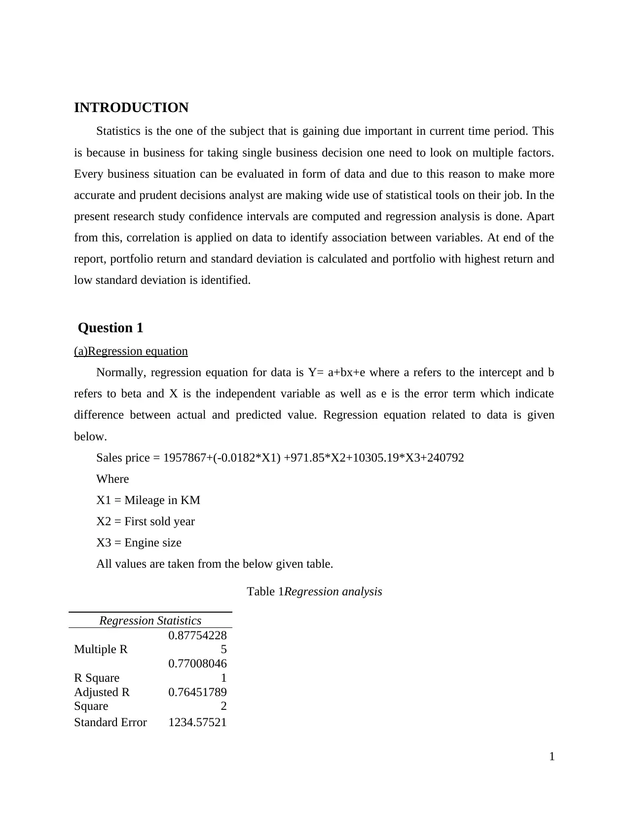
INTRODUCTION
Statistics is the one of the subject that is gaining due important in current time period. This
is because in business for taking single business decision one need to look on multiple factors.
Every business situation can be evaluated in form of data and due to this reason to make more
accurate and prudent decisions analyst are making wide use of statistical tools on their job. In the
present research study confidence intervals are computed and regression analysis is done. Apart
from this, correlation is applied on data to identify association between variables. At end of the
report, portfolio return and standard deviation is calculated and portfolio with highest return and
low standard deviation is identified.
Question 1
(a)Regression equation
Normally, regression equation for data is Y= a+bx+e where a refers to the intercept and b
refers to beta and X is the independent variable as well as e is the error term which indicate
difference between actual and predicted value. Regression equation related to data is given
below.
Sales price = 1957867+(-0.0182*X1) +971.85*X2+10305.19*X3+240792
Where
X1 = Mileage in KM
X2 = First sold year
X3 = Engine size
All values are taken from the below given table.
Table 1Regression analysis
Regression Statistics
Multiple R
0.87754228
5
R Square
0.77008046
1
Adjusted R
Square
0.76451789
2
Standard Error 1234.57521
1

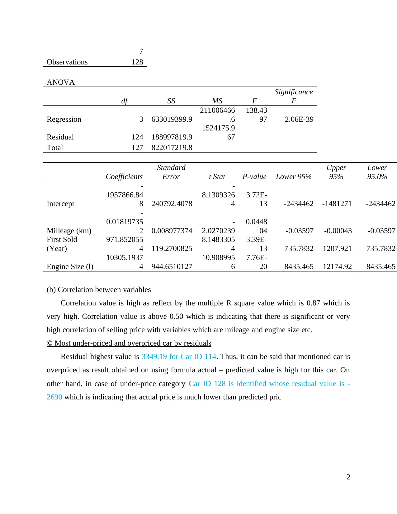
7
Observations 128
ANOVA
df SS MS F
Significance
F
Regression 3 633019399.9
211006466
.6
138.43
97 2.06E-39
Residual 124 188997819.9
1524175.9
67
Total 127 822017219.8
Coefficients
Standard
Error t Stat P-value Lower 95%
Upper
95%
Lower
95.0%
Intercept
-
1957866.84
8 240792.4078
-
8.1309326
4
3.72E-
13 -2434462 -1481271 -2434462
Milleage (km)
-
0.01819735
2 0.008977374
-
2.0270239
0.0448
04 -0.03597 -0.00043 -0.03597
First Sold
(Year)
971.852055
4 119.2700825
8.1483305
4
3.39E-
13 735.7832 1207.921 735.7832
Engine Size (l)
10305.1937
4 944.6510127
10.908995
6
7.76E-
20 8435.465 12174.92 8435.465
(b) Correlation between variables
Correlation value is high as reflect by the multiple R square value which is 0.87 which is
very high. Correlation value is above 0.50 which is indicating that there is significant or very
high correlation of selling price with variables which are mileage and engine size etc.
© Most under-priced and overpriced car by residuals
Residual highest value is 3349.19 for Car ID 114. Thus, it can be said that mentioned car is
overpriced as result obtained on using formula actual – predicted value is high for this car. On
other hand, in case of under-price category Car ID 128 is identified whose residual value is -
2690 which is indicating that actual price is much lower than predicted pric
2

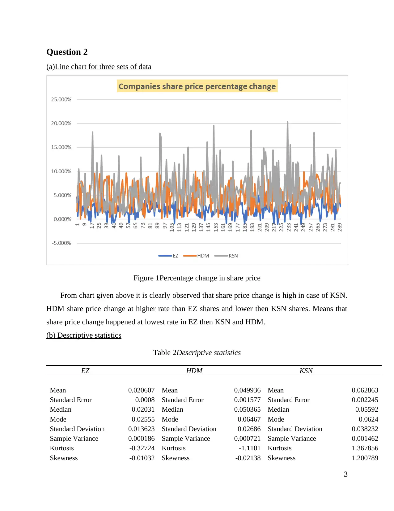
Question 2
(a)Line chart for three sets of data
Figure 1Percentage change in share price
From chart given above it is clearly observed that share price change is high in case of KSN.
HDM share price change at higher rate than EZ shares and lower then KSN shares. Means that
share price change happened at lowest rate in EZ then KSN and HDM.
(b) Descriptive statistics
Table 2Descriptive statistics
EZ HDM KSN
Mean 0.020607 Mean 0.049936 Mean 0.062863
Standard Error 0.0008 Standard Error 0.001577 Standard Error 0.002245
Median 0.02031 Median 0.050365 Median 0.05592
Mode 0.02555 Mode 0.06467 Mode 0.0624
Standard Deviation 0.013623 Standard Deviation 0.02686 Standard Deviation 0.038232
Sample Variance 0.000186 Sample Variance 0.000721 Sample Variance 0.001462
Kurtosis -0.32724 Kurtosis -1.1101 Kurtosis 1.367856
Skewness -0.01032 Skewness -0.02138 Skewness 1.200789
3

Range 0.06772 Range 0.09963 Range 0.19795
Minimum -0.01042 Minimum 0.00067 Minimum 0.00505
Maximum 0.0573 Maximum 0.1003 Maximum 0.203
Sum 5.97594 Sum 14.48151 Sum 18.23033
Count 290 Count 290 Count 290
Table 3Correlation analysis
EZ HDM KSN
EZ 1
HDM -0.01823 1
KSN 0.083413
-
0.01834 1
© Interpretation of data
From table above, it can be seen that in case of company EZ mean value is 2% with SD
of 0.013 and maximum value is 9.95 as well as minimum value is -0.01. So, on an average EZ
generate return of 2% and maximum return generate by company share is 9% while lowest return
is -0.1%. Standard deviation value is low for the firm. In case of HDM mean value is 4% and SD
is 0.02 followed by highest value is 1% and lowest is 0%. Hence, it can be said that return is
quite low in case of HDM. In case of KSN mean value is 6% followed by SD of 0.03 and
maximum value is 20% with lowest return of 0%. Thus, it can be said that KSN is generating
good return for investors.
Correlation is the value that is reflecting association between both multiple variables. It
can be seen that correlation value -0.01 for EZ and HDM. Hence, it can be said that both firm’s
stocks are negatively correlated to each other. On other hand in case of EZ and KSN correlation
value is 0.08 which is low correlation value. Hence, it can be said that there is no correlation
between these firms shares performance in the market.
4

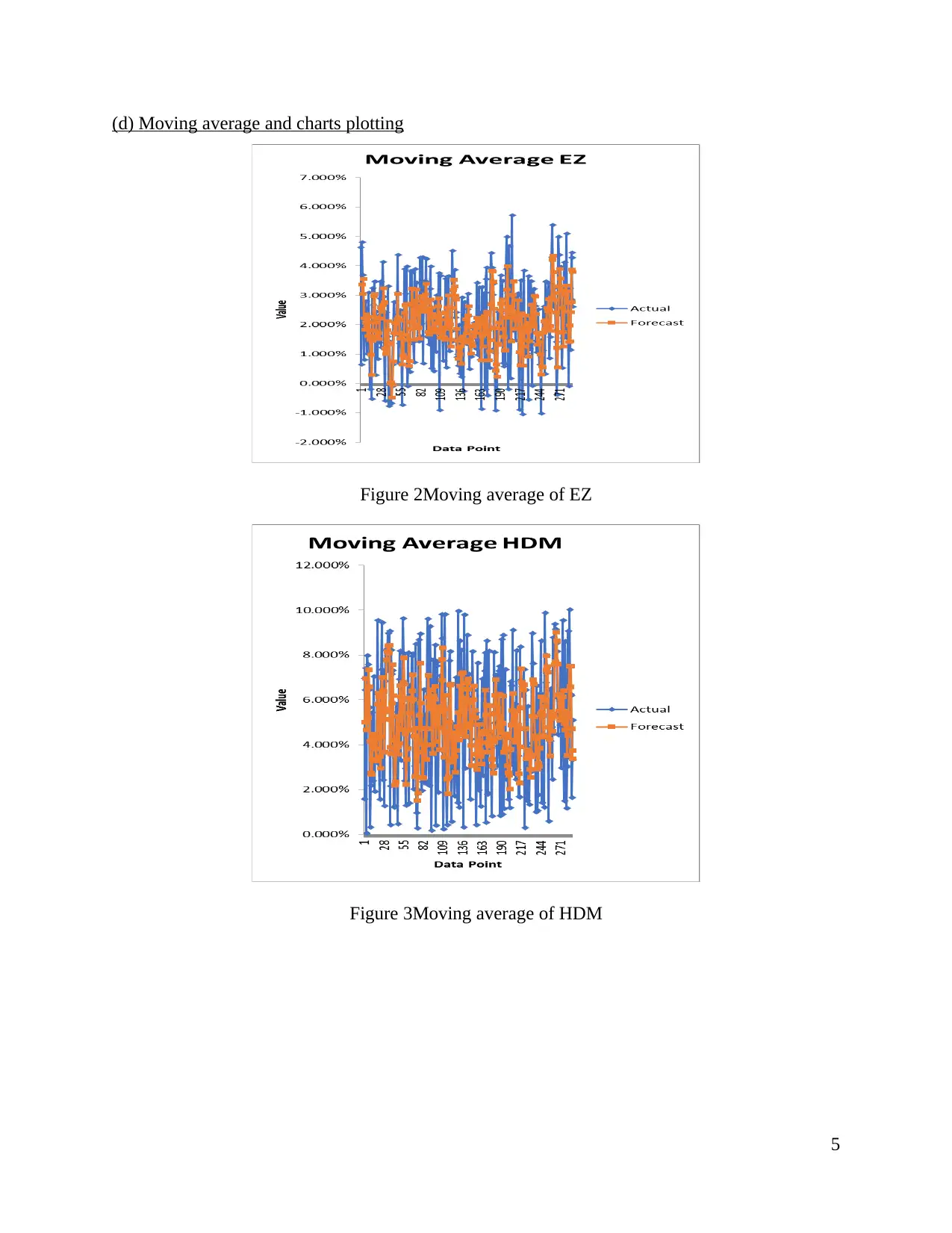
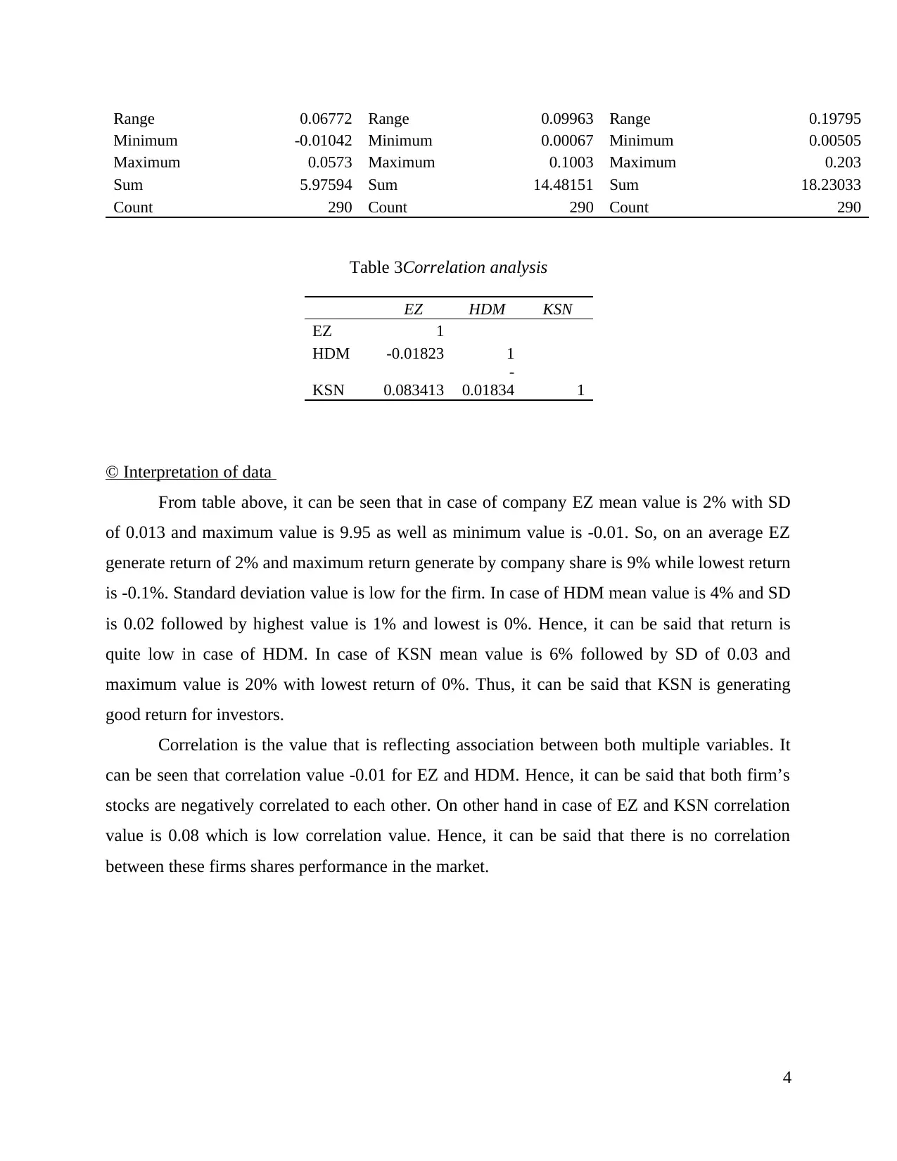
(d) Moving average and charts plotting
Figure 2Moving average of EZ
Figure 3Moving average of HDM
5

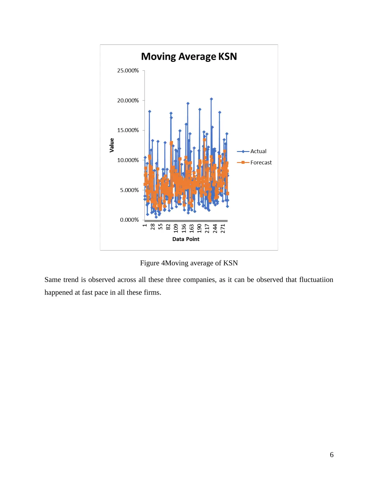
Figure 4Moving average of KSN
Same trend is observed across all these three companies, as it can be observed that fluctuatiion
happened at fast pace in all these firms.
6

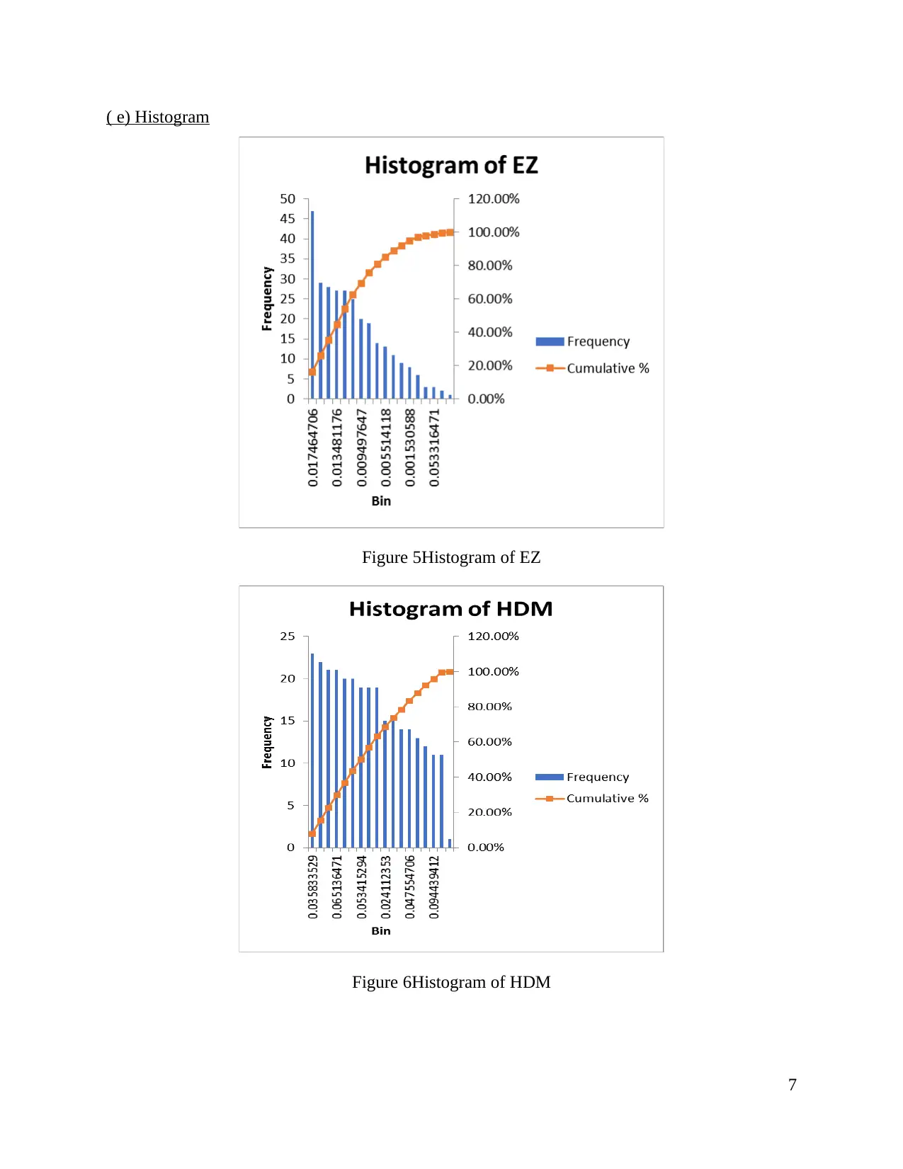
( e) Histogram
Figure 5Histogram of EZ
Figure 6Histogram of HDM
7

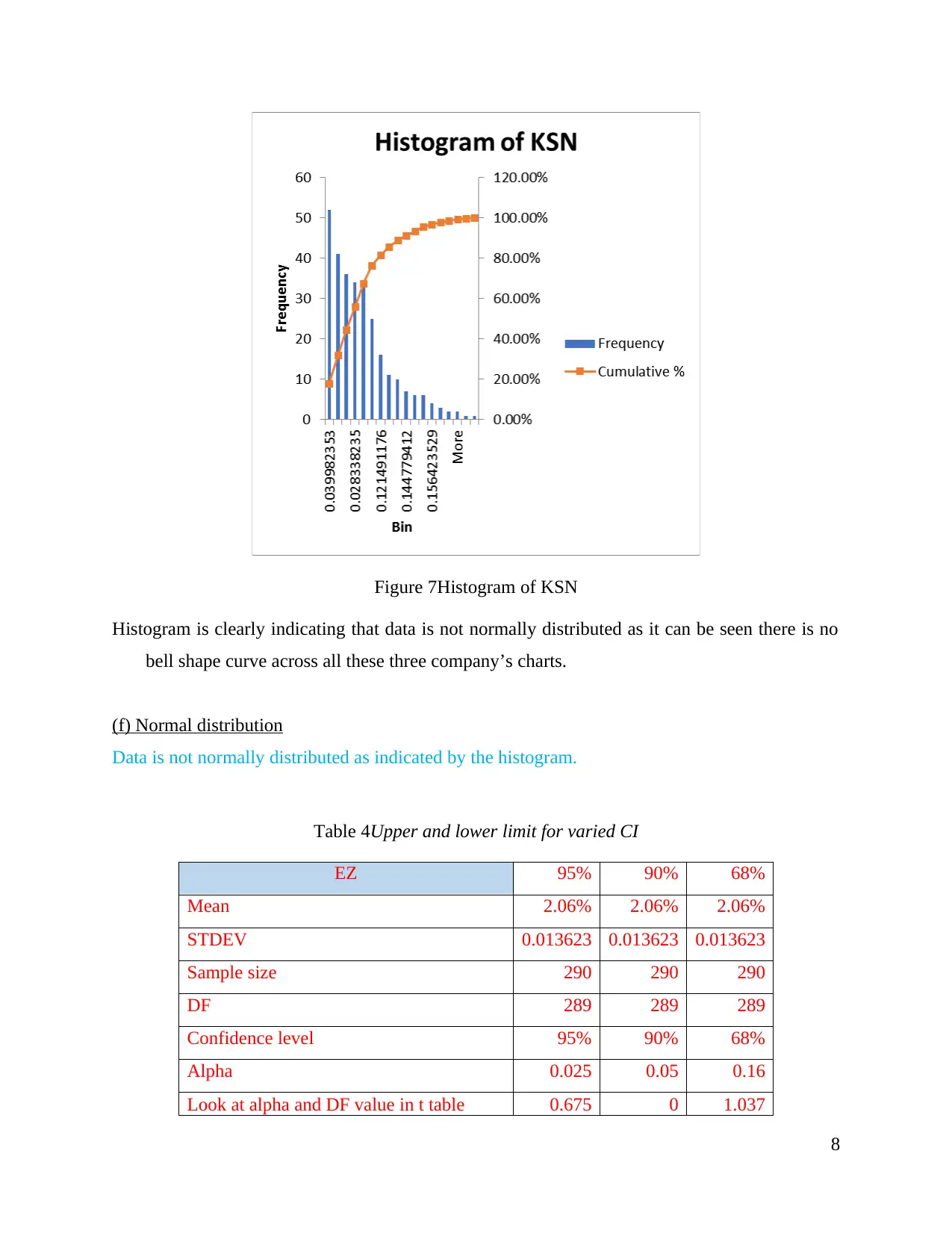
Figure 7Histogram of KSN
Histogram is clearly indicating that data is not normally distributed as it can be seen there is no
bell shape curve across all these three company’s charts.
(f) Normal distribution
Data is not normally distributed as indicated by the histogram.
Table 4Upper and lower limit for varied CI
EZ 95% 90% 68%
Mean 2.06% 2.06% 2.06%
STDEV 0.013623 0.013623 0.013623
Sample size 290 290 290
DF 289 289 289
Confidence level 95% 90% 68%
Alpha 0.025 0.05 0.16
Look at alpha and DF value in t table 0.675 0 1.037
8

STDEV/SQRT (Sample size) 0.0008 0.0008 0.0008
T table value* (STDEV/SQRT(Sample
size)) 0.00054 0 0.00083
Lower level 2.01% 2.06% 1.98%
Upper level 2.11% 2.06% 2.14%
HDM 95% 90% 68%
Mean 4.99% 4.99% 4.99%
STDEV 0.02686 0.02686 0.02686
Sample size 290 290 290
DF 289 289 289
Confidence level 95% 90% 68%
Alpha 0.025 0.05 0.16
Look at alpha and DF value in t table 0.675 0 1.037
STDEV/SQRT (Sample size) 0.001577 0.001577 0.001577
T table value* (STDEV/SQRT (Sample
size)) 0.001065 0 0.001636
Lower level 4.89% 4.99% 4.83%
Upper level 5.10% 4.99% 5.16%
KSN 95% 90% 68%
Mean 6.29% 6.29% 6.29%
STDEV 0.038232 0.038232 0.038232
Sample size 290 290 290
DF 289 289 289
Confidence level 95% 90% 68%
Alpha 0.025 0.05 0.16
Look at alpha and DF value in t table 0.675 0 1.037
STDEV/SQRT(Sample size) 0.002245 0.002245 0.002245
9

T table value* (STDEV/SQRT(Sample
size)) 0.001515 0 0.002328
Lower level 6.13% 6.29% 6.05%
Upper level 6.44% 6.29% 6.52%
Question 3
Identification of difference between A and B, B and C
H0: There is no significant difference between group A and B.
H1: There is no significant difference between group A and B.
Table 5T Test
t-Test: Two-Sample Assuming Unequal Variances
Group A Group B
Mean 0.033161 0.024867
Variance 7.9E-05 1.12E-05
Observations 18 15
Hypothesized Mean Difference 0
df 22
t Stat 3.65993
P(T<=t) one-tail 0.000689
t Critical one-tail 1.717144
P(T<=t) two-tail 0.001377
t Critical two-tail 2.073873
Interpretation
From the table given above it can be seen that value of level of significance is 0.00<0.05
which is indicating that there is significant difference between both group A and B. Both groups
are independent of each other and it can be said that T test selected for testing purpose is wise
decision.
H0: There is no significant difference between group B and C.
H1: There is no significant difference between group B and C.
10

Table 6 T Test
t-Test: Two-Sample Assuming Unequal Variances
Group B Group C
Mean 0.024867 0.022753
Variance 1.12E-05 2.77E-05
Observations 15 17
Hypothesized Mean Difference 0
df 27
t Stat 1.371062
P(T<=t) one-tail 0.090823
t Critical one-tail 1.703288
P(T<=t) two-tail 0.181645
t Critical two-tail 2.051831
Interpretation
Value of level of significance is 0.29> 0.05 which is indicating that there is no significant
difference between both groups which are B and C.
Question 4
(a)Calculating confidence interval
Table 7CI calculation
CI of investment 95% 90% 68%
Mean 12357 12357 12357
STDEV 2403.810497 2403.810497 2403.810497
Sample size 30 30 30
DF 29 29 29
Confidence level 95% 90% 68%
Alpha 0.025 0.05 0.16
Look at alpha and DF value in t table 0.675 0 1.037
STDEV/SQRT(Sample size) 438.8737444 438.8737444 438.8737444
T table value* (STDEV/SQRT(Sample
size)) 296.2397775 0 455.112073
Lower level 12060.46 12356.70 11901.59
11

Upper level 12652.94 12356.70 12811.81
(b) Z test
H0: There is no difference between average value and given value.
H1: There is difference between average value and given value.
Table 8Z test calculation
X 12356.70
Mu 11500
STDEV 2550
Z test 0.335960784
Interpretation
From table it can be seen that Z test value is 0.33 when we find value in Z table by
considering this confidence level is 0.62 or 62%. Hence, value does not reach to 95% and 99%
confidence level. Hence, it can be said null hypothesis accepted.
© Performance of test
No difference is observed in results.
Question 5
H0: There is not significant difference between type and amount in terms of variance exists
between them.
H1: There is significant difference between type and amount in terms of variance exists between
them.
Table 9ANNOVA
Anova: Single Factor
SUMMARY
Groups Count Sum Average Variance
Type 137 207 1.510949 0.251717
Amount 137 273 1.992701 0.727888
12

ANOVA
Source of
Variation SS df MS F
P-
value F crit
Between
Groups 15.89781 1 15.89781 32.45759
3.16E-
08 6.728965
Within Groups 133.2263 272 0.489802
Total 149.1241 273
Interpretation
On basis of results it is identified that there is no significant difference in terms of
variance between groups which are type of investment and amount invested. Value of level of
significance is 3.16>0.05. Means that with change in investment type amount invested does not
change significantly.
H0: There is no significant difference between amount and day in terms of variance.
H1: There is significant difference between amount and day in terms of variance.
Table 10ANNOVA
Anova: Single
Factor
SUMMARY
Groups Count Sum Average Variance
Amount 147 297 2.020408 0.732457
Day 147 382 2.598639 1.419998
ANOVA
Source of
Variation SS df MS F
P-
value F crit
Between Groups 24.57483 1 24.57483 22.83423
2.8E-
06 6.722461
Within Groups 314.2585 292 1.076228
Total 338.8333 293
Interpretation
13

Value of level of significance is 2.8>0.05 which is indicating that there is no significant
difference between both factors. Hence, it can be said that with change in days of week no big
change comes in investment amount.
Question 6
(a)
(a)
Table 11Expected return and STDEV of portfolio
A Weight 20%
B weight 80%
Return on A 2%
Return on B 2.30%
Expected return 2.2400%
A Weight 20%
B weight 80%
STDEV A 0.20%
STDEV B 0.40%
Correlation A and
B 0.3
Variance 0.000011168
STDEV of
portfolio 0.33%
(b)
Table 12Return and STDEV of portfolio with 3 stocks
A Weight 50%
B Weight 30%
C Weight 20%
Return on A 2%
Return on B 2.30%
Return on C 1.50%
A Weight 50%
14

B weight 30%
C Weight 20%
STDEV A 0.20%
STDEV B 0.40%
STDEV C 1%
Variance 0.00000972
STDEV of
portfolio 0.31%
(b)
Table 13Portfolio analysis
Portfolio of A and B Portfolio of B and C Portfolio of C and A
A Weight 40% B Weight 80% C Weight 40%
B weight 60% C weight 20% A weight 60%
Return on A 2% Return on B 2% Return on C 2%
Return on B 2.30% Return on C 1.50% Return on A 2.00%
Expected return 2.1800% Expected return 2.1400% Expected return
1.8000
%
A Weight 20% B Weight 20% C Weight 40%
B weight 80% C weight 80% A weight 60%
STDEV A 0.20% STDEV B 0.40% STDEV C 1.00%
STDEV B 0.40% STDEV C 1.00% STDEV A 0.20%
Correlation A
and B 0.3
Correlation B
and C 0.2
Correlation C
and A 0.4
Variance
0.0000111
68 Variance
0.00006
72 Variance
2.13E-
05
STDEV of
portfolio 0.33%
STDEV of
portfolio 0.82%
STDEV of
portfolio 0.46%
Maximum return is observed in case of portfolio of A and B where weight of A is 40%
and same of B is 60%. Standard deviation is also very low in case of portfolio A and B where
value of statistic is 0.33% which is lower than another portfolio’s. Minimum return is observed
in case portfolio C and A where return percentage is 1.8%. Maximum standard deviation is
observed in case of portfolio B and C where its value is 0.82%.
15

Question 7
Statistics now a days is used for data analysis purpose to great extent. In earlier time period
normally in the stock market line charts were analyzed. In advanced level candelstick charts
were anlyzed, but now a days stock analysts are widely using statistics in order to deep dive in
data and identifying meaningful patterns which support decision making process. There is huge
scope of statistics and one need to focus on lots of things in order to bring out meaningful and
true conclusion. Many times analysts make use of wrong tools to analyze data or sometimes
failed to prerpare data set for the specific statisitcal tool so that better decisions can be made at
workplace (Adam, Marcet and Nicolini, 2016). This can be understand from speciofic example
like in data analytics huge stress is laid down on data cleaning. It can be noted that many time
data is unstructured or there are lots of outliers in them. It is very important to understand term
outlier before move forward. Outlier refers to the extremely upper or lower values that are almost
out of range. This can be understand from another example like we seen in line charts where
soemtimes there are huge spikes in terms of upward and downward trend. Such kind of spikes
that are extremely high and low are considered as outlier. It is very important to remove these
outliers from the data set so that reliable predictions can be made on the basis of statistical
model. In case outliers will not be removed then in that case these extreme high and low points
will influence results. Many times analyst who is not so perfect in data science directly make use
of raw data for preparing regression model. In such kind of situation. Wrong results are produced
by model and analyse make wrong decisions.
Many times it is observed that analyst make use of wrong methods to analyze data and
make wrong interpretation. In such kind of scenerio analyst want to arrive at specific result and
he think that whatever method it used is accurate. In case of such kind of situatiion analyst make
wrong conclusions and make wrong decisions. Thus, where tool can be applied and what sort of
data is required by tool to generate accurate results are some of questions whose answers analyst
must know (Almenberg and Dreber, 2015). Use of unreliable data is another major problem
associated with data analysis of stock market data and making business decisions. Interesting to
note is that stock market keeps on fluctuating on regular basis. Hence, duration upto which
analyst is taking data have key importance from analysis point of view. Just suppose analyst take
last one month data to make investment deciions for upcomuing three months then such kind of
act can generate huge risk for individual. This is because just be analyzing one month data
16

accurate results can not be obtained. One atleast need to analyze past three months data so that
accurate overview of the current market can be obtained. Thus, such kind of data inaccuracies
are the major issues associated with use of statistical approaches in making invesment decisions.
This does not mean that there are numbe of conditions one have to fulfill and due to this reason it
become hard to get accurate results from the statistical tools.
One if satisfy all conditions then in that case it can get accurate results on application of
tools like regression analysis. By using this tool it can be identified that to what extent index
affect stock performance and what percentage of the variation of the company stock is explained
by the index. Thus, on basis of results one can identify extent to which index is affecting stock
performance. If percentage of variation explained is less then it can be concluded that stock and
index to some extent move at different rate in same direction. Reaosn may by multiple like poor
performance of the company etc. Thus, by using such kind of method in better way investor can
make decisions. It can be said that there are both positive and negative side of use of statistical
methods for making stock market decisions.
Suppose analyst take data related to appropriate time period then in that situaton also analyst
need to ensuure that data is normally distributed and parametric test can be applied. In order to
check normal distribution histogram can be prepared where bell shape curve clearly indicate
whether data is normally distributed. Thus, by taking right time period data which is normally
distributed by using statistical tools better decisions can be taken by the analyst at the workplace.
Results interpretation is the another area where analysts makes a lot of mistakes (Sutcliffe,
2018). Statistical tools are technical things and one need to be fully aware about concepts like
confidence level etc. Due to lack of absense of proper knowledge expert can make wrong
business decisions. Apart from this, it can be noted that in tool like regression analysis lots of
facts are available which are reflecting different things like multiple R, P value and residuals etc
(Patel and et.al., 2015). Many time analyst analyze and interpret one thing in right way and othe
thing in wrong manner. In such kind of situation there is huge probability of making wrong
decisions. Thus, stock analyst need to make use of all informations together and need to
coorleate them in proper manner so that overall picture can be viewed (Statistics problems.,
2019). Hence, it can be said that there are lots of issues associated with use of statistical tools in
terms of their use and facts interpretation and due to this reason one need to have deep
17

knowledge of tools and techniques. Apart from this, one need to ensure that data used in
parametric test is normally distributed. Hence, overall due care need to be taken.
CONCLUSION
On basis of above discussion, it is concluded that there is significant importance of statistical
tools for the business people because this help them in looking in multiple areas so that better
business decisions can be made. Before making use of statistical tools one need to ensure that
data quality is perfect and it had passed all parameters. Along with this, it must be ensured that
data is taken from reliable sources by the business firm. Analyst also need to ensure that right
tool is used for data analysis purpose. By doing all these things prudent decisions can be taken by
analyst.
18

REFERENCES
Books and Journals
Adam, K., Marcet, A. and Nicolini, J.P., 2016. Stock market volatility and learning. The Journal
of Finance. 71(1). pp.33-82.
Almenberg, J. and Dreber, A., 2015. Gender, stock market participation and financial
literacy. Economics Letters. 137. pp.140-142.
Patel, J and et.al., 2015. Predicting stock market index using fusion of machine learning
techniques. Expert Systems with Applications. 42(4). pp.2162-2172.
Sutcliffe, C.M., 2018. Stock index futures. Routledge.
Online
Statistics problems., 2019. [Online]. Available through:<
https://stattrek.com/statistics/problems.aspx>.
19