Quantitative Methods Assignment: Statistical Analysis & Solutions

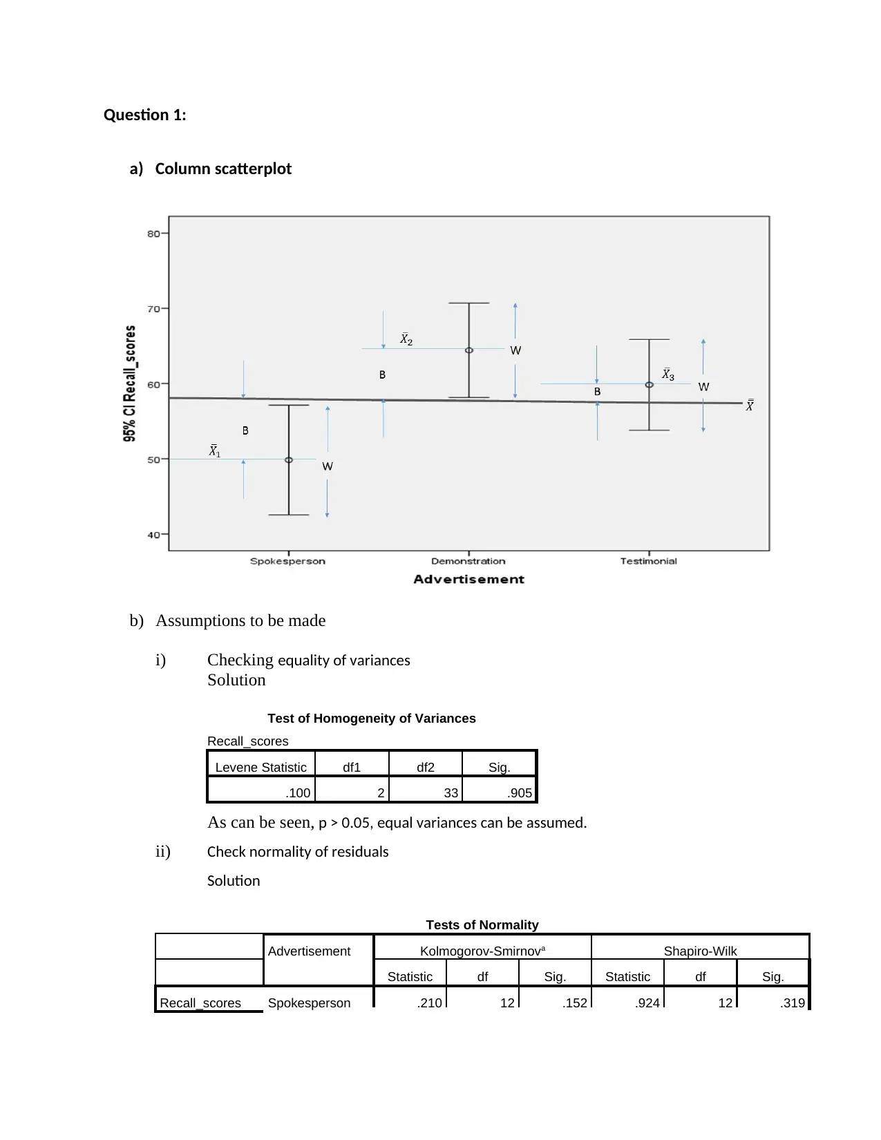
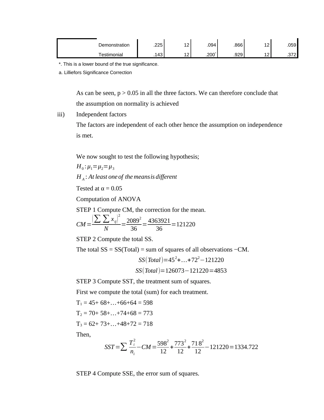
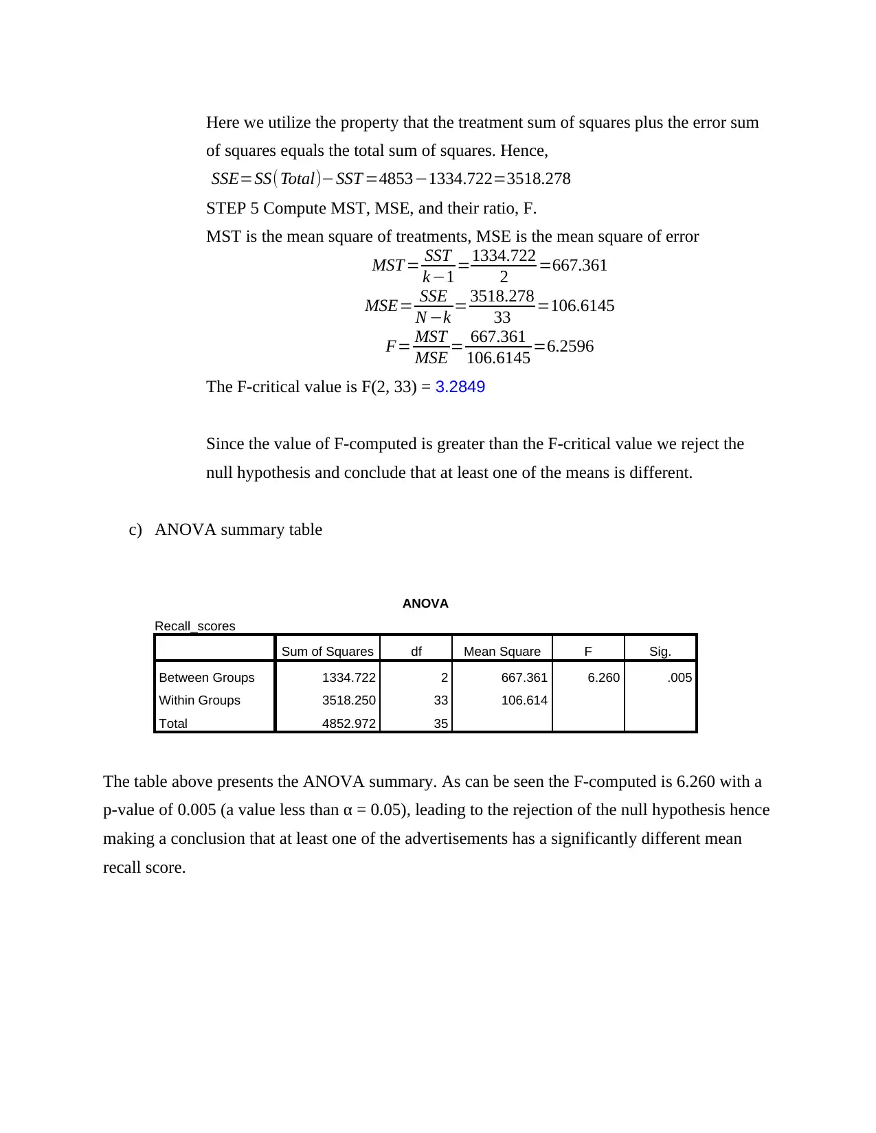
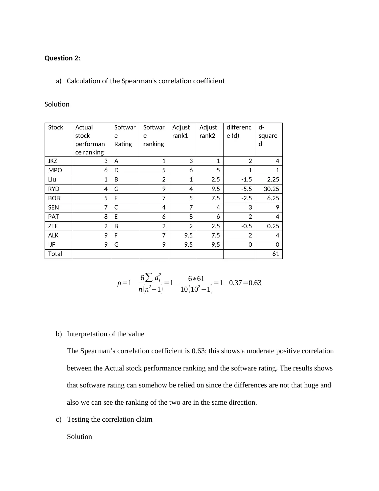
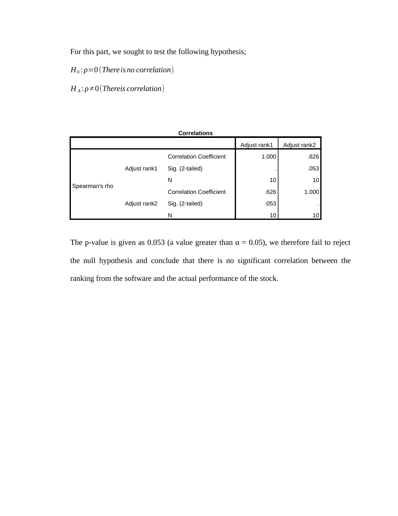
This document presents a comprehensive solution to a Quantitative Methods assignment, addressing two main questions. The first question involves analyzing advertisement recall scores using ANOVA. The solution includes checking assumptions such as equality of variances and normality of residuals, followed by the computation of ANOVA to determine if there are significant differences in recall scores among different advertisement types. The second question focuses on calculating the Spearman's correlation coefficient to assess the relationship between software ratings and actual stock performance rankings. The solution involves ranking the data, computing the coefficient, and testing the correlation claim using hypothesis testing to determine the statistical significance of the relationship. The document provides detailed calculations, interpretations, and conclusions for both questions, offering a clear understanding of the statistical methods applied.

Quantitative Methods
Student name:
University
Lecturer name:
13th October 2017

Question 1:
a) Column scatterplot
b) Assumptions to be made
i) Checking equality of variances
Solution
Test of Homogeneity of Variances
Recall_scores
Levene Statistic df1 df2 Sig.
.100 2 33 .905
As can be seen, p > 0.05, equal variances can be assumed.
ii) Check normality of residuals
Solution
Tests of Normality
Advertisement Kolmogorov-Smirnova Shapiro-Wilk
Statistic df Sig. Statistic df Sig.
Recall_scores Spokesperson .210 12 .152 .924 12 .319

Demonstration .225 12 .094 .866 12 .059
Testimonial .143 12 .200* .929 12 .372
*. This is a lower bound of the true significance.
a. Lilliefors Significance Correction
As can be seen, p > 0.05 in all the three factors. We can therefore conclude that
the assumption on normality is achieved
iii) Independent factors
The factors are independent of each other hence the assumption on independence
is met.
We now sought to test the following hypothesis;
H0 : μ1=μ2=μ3
H A : At least one of the meansis different
Tested at α = 0.05
Computation of ANOVA
STEP 1 Compute CM, the correction for the mean.
CM = (∑ ∑ xij )2
N =20892
36 = 4363921
36 =121220
STEP 2 Compute the total SS.
The total SS = SS(Total) = sum of squares of all observations −CM.
SS(Total )=452+ …+722−121220
SS(Total )=126073−121220=4853
STEP 3 Compute SST, the treatment sum of squares.
First we compute the total (sum) for each treatment.
T1 = 45+ 68+…+66+64 = 598
T2 = 70+ 58+…+74+68 = 773
T3 = 62+ 73+…+48+72 = 718
Then,
SST =∑ T i
2
ni
−CM =5982
12 + 7732
12 +71 82
12 −121220=1334.722
STEP 4 Compute SSE, the error sum of squares.

Here we utilize the property that the treatment sum of squares plus the error sum
of squares equals the total sum of squares. Hence,
SSE=SS( Total)−SST =4853−1334.722=3518.278
STEP 5 Compute MST, MSE, and their ratio, F.
MST is the mean square of treatments, MSE is the mean square of error
MST = SST
k −1 =1334.722
2 =667.361
MSE= SSE
N −k = 3518.278
33 =106.6145
F= MST
MSE = 667.361
106.6145 =6.2596
The F-critical value is F(2, 33) = 3.2849
Since the value of F-computed is greater than the F-critical value we reject the
null hypothesis and conclude that at least one of the means is different.
c) ANOVA summary table
ANOVA
Recall_scores
Sum of Squares df Mean Square F Sig.
Between Groups 1334.722 2 667.361 6.260 .005
Within Groups 3518.250 33 106.614
Total 4852.972 35
The table above presents the ANOVA summary. As can be seen the F-computed is 6.260 with a
p-value of 0.005 (a value less than α = 0.05), leading to the rejection of the null hypothesis hence
making a conclusion that at least one of the advertisements has a significantly different mean
recall score.

Question 2:
a) Calculation of the Spearman's correlation coefficient
Solution
Stock Actual
stock
performan
ce ranking
Softwar
e
Rating
Softwar
e
ranking
Adjust
rank1
Adjust
rank2
differenc
e (d)
d-
square
d
JKZ 3 A 1 3 1 2 4
MPO 6 D 5 6 5 1 1
Llu 1 B 2 1 2.5 -1.5 2.25
RYD 4 G 9 4 9.5 -5.5 30.25
BOB 5 F 7 5 7.5 -2.5 6.25
SEN 7 C 4 7 4 3 9
PAT 8 E 6 8 6 2 4
ZTE 2 B 2 2 2.5 -0.5 0.25
ALK 9 F 7 9.5 7.5 2 4
IJF 9 G 9 9.5 9.5 0 0
Total 61
ρ=1− 6∑ di
2
n ( n2−1 ) =1− 6∗61
10 ( 102 −1 ) =1−0.37=0.63
b) Interpretation of the value
The Spearman’s correlation coefficient is 0.63; this shows a moderate positive correlation
between the Actual stock performance ranking and the software rating. The results shows
that software rating can somehow be relied on since the differences are not that huge and
also we can see the ranking of the two are in the same direction.
c) Testing the correlation claim
Solution

For this part, we sought to test the following hypothesis;
H0 : ρ=0 (Thereis no correlation)
H A : ρ ≠ 0(Thereis correlation)
Correlations
Adjust rank1 Adjust rank2
Spearman's rho
Adjust rank1
Correlation Coefficient 1.000 .626
Sig. (2-tailed) . .053
N 10 10
Adjust rank2
Correlation Coefficient .626 1.000
Sig. (2-tailed) .053 .
N 10 10
The p-value is given as 0.053 (a value greater than α = 0.05), we therefore fail to reject
the null hypothesis and conclude that there is no significant correlation between the
ranking from the software and the actual performance of the stock.