BEA140 Quantitative Methods Assignment: Solutions and Analysis
VerifiedAdded on 2020/05/04
|9
|2886
|285
Homework Assignment
AI Summary
This document presents the complete solutions to a Quantitative Methods assignment (BEA140), encompassing two main questions. The first question focuses on analyzing the product recall associated with different TV infomercials using ANOVA. It includes creating a multi-vari chart, testing hypotheses about the variation in recall scores, summarizing calculations in an ANOVA table, and interpreting the results, including addressing a marketing manager's claim. The second question involves analyzing customer perception of monorail cleanliness using a chi-square test to determine if cleanliness is independent of the monorail circuit. This includes hypothesis testing, calculating expected frequencies, determining degrees of freedom, and explaining the difference between Type I and Type II errors, with examples relevant to the problem. All solutions include detailed calculations, interpretations, and conclusions based on the statistical tests performed.
Make Up Assignment (optional)
BEA140 Quantitative Methods
Semester 2, 2014
Due 4:00 pm, 17 October
Total Marks Available: 50
Contribution to final mark 5% (see page 4)
Section A: Attempt Question 1
Question 1
One of the key measures of the success of TV “infomercial” advertising is the amount of information that viewers can
recall about the advertised product.
The marketers of a new fat free cooking system have had three infomercials developed:
A spokesperson style advertisement featuring a celebrity,
A product demonstration style advertisement showing the product being used,
A testimonial style advertisement, featuring satisfied users.
They are wondering whether they are equally suited to day time television, in particular whether or not there is
significant variation in the level of product recall associated with the three advertisements. Their researchers compile
three random samples of day time television viewers – one sample for each advertisement. Each sample has 12
viewers. The viewers are shown their particular advertisement, and then are tested on their recall. Their recall scores
(out of 100) appear in the table below.
Spokesperson Demonstration Testimonial
45 70 62
68 58 73
49 75 46
51 54 48
45 49 59
49 72 56
37 75 71
48 57 55
29 70 64
47 51 64
66 74 48
64 68 72
a Present the data as a fully labelled “multi vari” chart of the form used on page two of the ANOVA handout. (NB
Hand drawn charts are acceptable. Novice users of Excel may find it easier to draw the chart by hand.)
[7 marks]
b Being careful to state any assumptions that you may need to make, test at the =0.10 level, whether product
recall varies across the infomercials. State your conclusions clearly. Include a reference citing where you obtained
the critical value.
[8+1+1=10 marks]
c Summarise your calculations using an ANOVA summary table.
[6 marks]
d The Marketing manager claims that this exercise proves that product demonstration causes increased Recall.
Explain whether the manager’s claim is correct.
[2 marks]
[Total: 25 marks]
1
Paraphrase This Document
Need a fresh take? Get an instant paraphrase of this document with our AI Paraphraser
Section B: Attempt Question 2
Question 2
The World Fair Monorail Company (WFMC) operates five monorail circuits, one in each of Shelbyville, Brockway and
Ogdenville, and two in Springfield (an older monorail and a newer one). Each month, as part of an ongoing customer
service monitor, a random selection of travellers are interviewed about their most recent monorail experience. One of
the questions asks the traveller to rate the monorail’s cleanliness. The most recent month’s results appear in the table
below.
Circuit
Cleanliness
Shelbyville Brockway Ogdenville Old Springfield New
Springfield
TOTAL
Satisfactory 28 29 43 22 7 129
Unsatisfactory 11 3 4 4 1 23
TOTAL 39 32 47 26 8 152
The management of WFMC wish to understand whether all of their monorails are performing equally well with
respect to perceived cleanliness. (That is, whether cleanliness is independent of circuit.)
a Being careful to state your conclusions, and using a level of significance of = 10%, test whether perception of
cleanliness is independent of circuit.
[21 marks]
b Explain the difference between a type 1 and type 2 error. Use this problem to provide examples.
[4 marks]
[Total: 25 marks]
Solutions
Answer 1.a
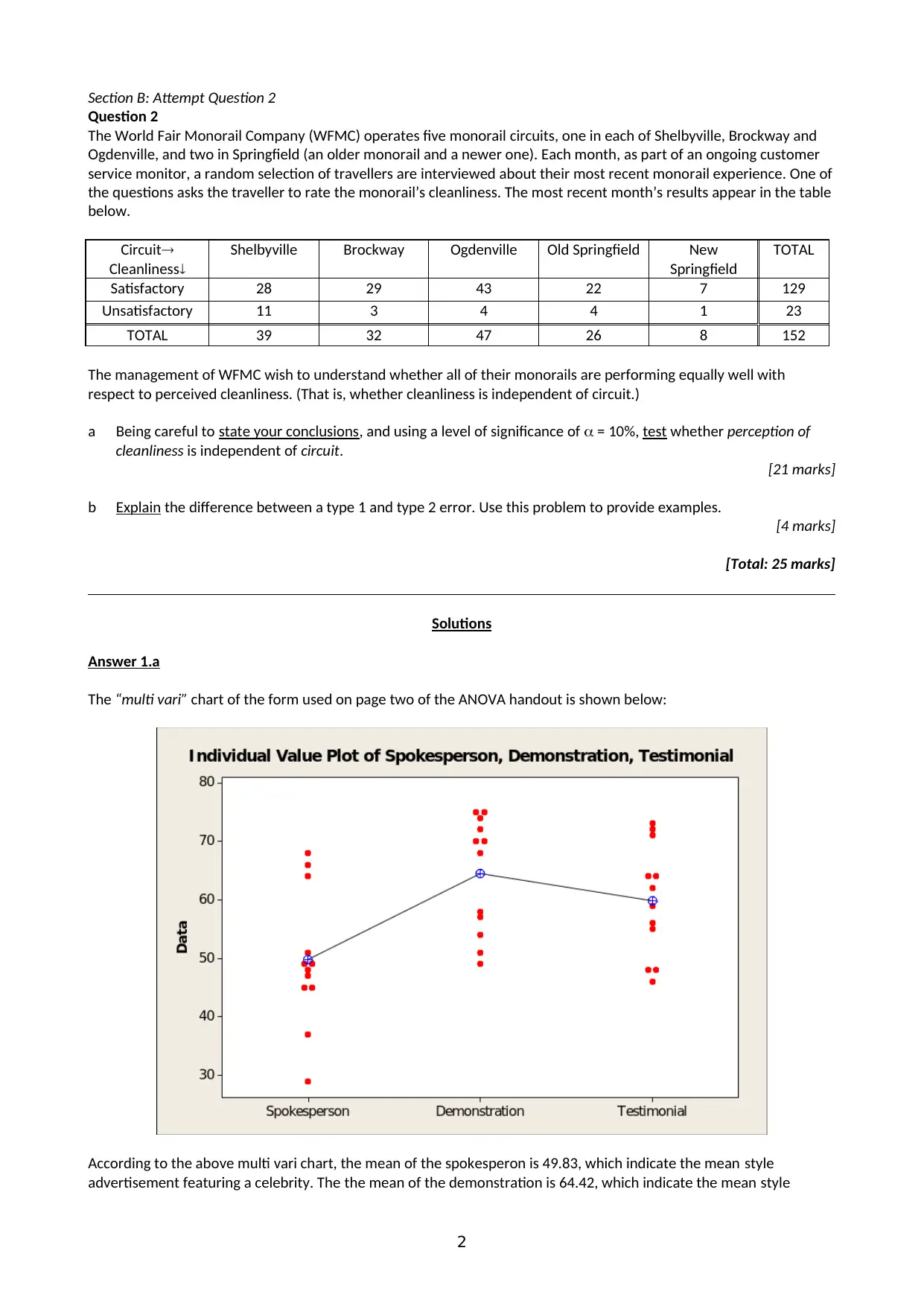
The “multi vari” chart of the form used on page two of the ANOVA handout is shown below:
According to the above multi vari chart, the mean of the spokesperon is 49.83, which indicate the mean style
advertisement featuring a celebrity. The the mean of the demonstration is 64.42, which indicate the mean style
2
Question 2
The World Fair Monorail Company (WFMC) operates five monorail circuits, one in each of Shelbyville, Brockway and
Ogdenville, and two in Springfield (an older monorail and a newer one). Each month, as part of an ongoing customer
service monitor, a random selection of travellers are interviewed about their most recent monorail experience. One of
the questions asks the traveller to rate the monorail’s cleanliness. The most recent month’s results appear in the table
below.
Circuit
Cleanliness
Shelbyville Brockway Ogdenville Old Springfield New
Springfield
TOTAL
Satisfactory 28 29 43 22 7 129
Unsatisfactory 11 3 4 4 1 23
TOTAL 39 32 47 26 8 152
The management of WFMC wish to understand whether all of their monorails are performing equally well with
respect to perceived cleanliness. (That is, whether cleanliness is independent of circuit.)
a Being careful to state your conclusions, and using a level of significance of = 10%, test whether perception of
cleanliness is independent of circuit.
[21 marks]
b Explain the difference between a type 1 and type 2 error. Use this problem to provide examples.
[4 marks]
[Total: 25 marks]
Solutions
Answer 1.a
The “multi vari” chart of the form used on page two of the ANOVA handout is shown below:
According to the above multi vari chart, the mean of the spokesperon is 49.83, which indicate the mean style
advertisement featuring a celebrity. The the mean of the demonstration is 64.42, which indicate the mean style
2
advertisement showing the product being used. The the mean of the testimonial is 59.83, which indicate the style
advertisement, featuring satisfied users.
Answer 1.b
Consider the provided details of 12 viewers of each sample who have been selected for three advertisements. The
level of product associated with the three advertisements, a spokesperson style advertisement featuring a celebrity, a
product demonstration style advertisement showing the product being used and a testimonial style advertisement,
featuring satisfied users. So there are three samples with three different conditions. So, the samples can be considerd
as independent. The condition of the independent level is also called a level or a treatment. And the difference
produced by the independent variable is called a treatment effect. The independent variables are called as between
subject factor. Hence, to heck the differences between sample means the one-way ANOVA will be used.
Assumptions for the one-way ANOVA are given as below:
1. Dependent variable should be measured at the interval or ratio level (Continuous).
2. Independent variable should be measured at the two or more categories.
3. There is no relationship between the observations of each group in independent variable.
4. There are no significant outliers.
5. Dependent variable should be normally distributed for each category if independent variable.
6. There needs of homogeneity of variance, so the Levene’s test will be applied for homogeneity of variance.
Consider the null and alternate hypothesis to test the claim, as given below:
Against the alternative hypothesis as shown below:
Here, , and are the means of, a spokesperson style advertisement featuring a celebrity, a product
demonstration style advertisement showing the product being used and a testimonial style advertisement featuring
satisfied users repectively. Consider the level of significance for the test as .
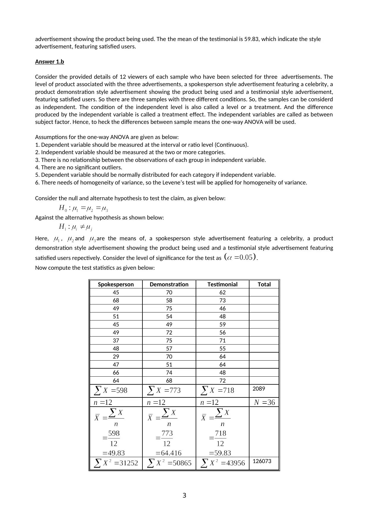
Now compute the test statistics as given below:
Spokesperson Demonstration Testimonial Total
45 70 62
68 58 73
49 75 46
51 54 48
45 49 59
49 72 56
37 75 71
48 57 55
29 70 64
47 51 64
66 74 48
64 68 72
2089
126073
3
advertisement, featuring satisfied users.
Answer 1.b
Consider the provided details of 12 viewers of each sample who have been selected for three advertisements. The
level of product associated with the three advertisements, a spokesperson style advertisement featuring a celebrity, a
product demonstration style advertisement showing the product being used and a testimonial style advertisement,
featuring satisfied users. So there are three samples with three different conditions. So, the samples can be considerd
as independent. The condition of the independent level is also called a level or a treatment. And the difference
produced by the independent variable is called a treatment effect. The independent variables are called as between
subject factor. Hence, to heck the differences between sample means the one-way ANOVA will be used.
Assumptions for the one-way ANOVA are given as below:
1. Dependent variable should be measured at the interval or ratio level (Continuous).
2. Independent variable should be measured at the two or more categories.
3. There is no relationship between the observations of each group in independent variable.
4. There are no significant outliers.
5. Dependent variable should be normally distributed for each category if independent variable.
6. There needs of homogeneity of variance, so the Levene’s test will be applied for homogeneity of variance.
Consider the null and alternate hypothesis to test the claim, as given below:
Against the alternative hypothesis as shown below:
Here, , and are the means of, a spokesperson style advertisement featuring a celebrity, a product
demonstration style advertisement showing the product being used and a testimonial style advertisement featuring
satisfied users repectively. Consider the level of significance for the test as .
Now compute the test statistics as given below:
Spokesperson Demonstration Testimonial Total
45 70 62
68 58 73
49 75 46
51 54 48
45 49 59
49 72 56
37 75 71
48 57 55
29 70 64
47 51 64
66 74 48
64 68 72
2089
126073
3
⊘ This is a preview!⊘
Do you want full access?
Subscribe today to unlock all pages.
Trusted by 1+ million students worldwide
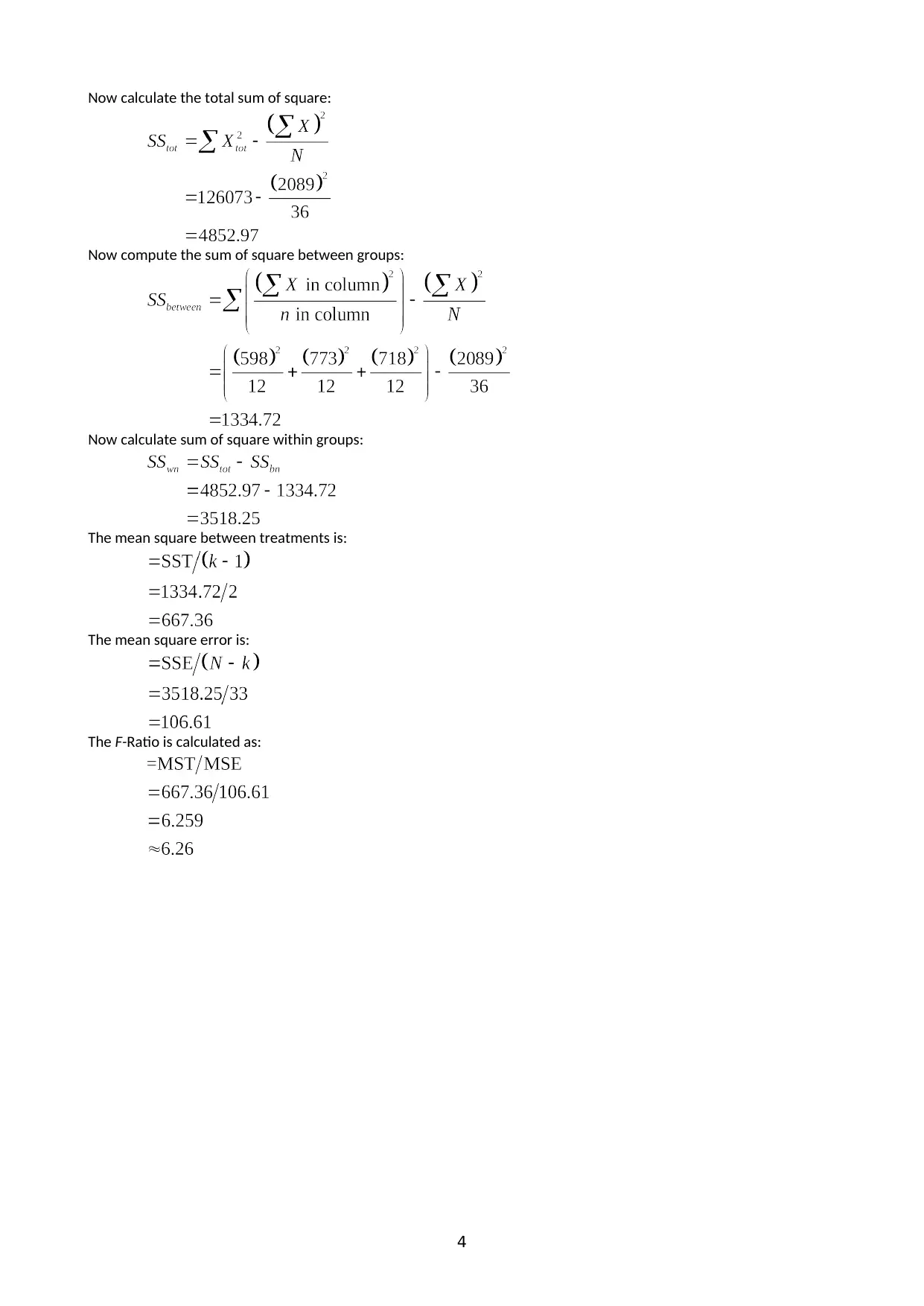
Now calculate the total sum of square:
Now compute the sum of square between groups:
Now calculate sum of square within groups:
The mean square between treatments is:
The mean square error is:
The F-Ratio is calculated as:
4
Now compute the sum of square between groups:
Now calculate sum of square within groups:
The mean square between treatments is:
The mean square error is:
The F-Ratio is calculated as:
4
Paraphrase This Document
Need a fresh take? Get an instant paraphrase of this document with our AI Paraphraser
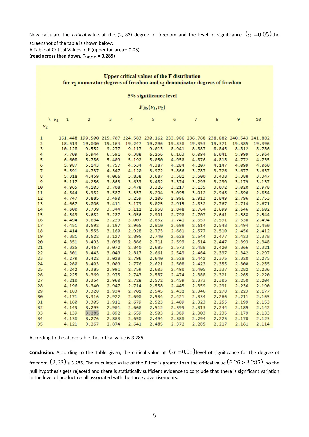
Now calculate the critical-value at the (2, 33) degree of freedom and the level of significance the
screenshot of the table is shown below:
A Table of Critical Values of F (upper tail area = 0.05)
(read across then down, F0.05,2,33 = 3.285)
According to the above table the critical value is 3.285.
Conclusion: According to the Table given, the critical value at level of significance for the degree of
freedom is 3.285. The calculated value of the F-test is greater than the critical value , so the
null hypothesis gets rejecetd and there is statistically sufficient evidence to conclude that there is significant variation
in the level of product recall associated with the three advertisements.
5
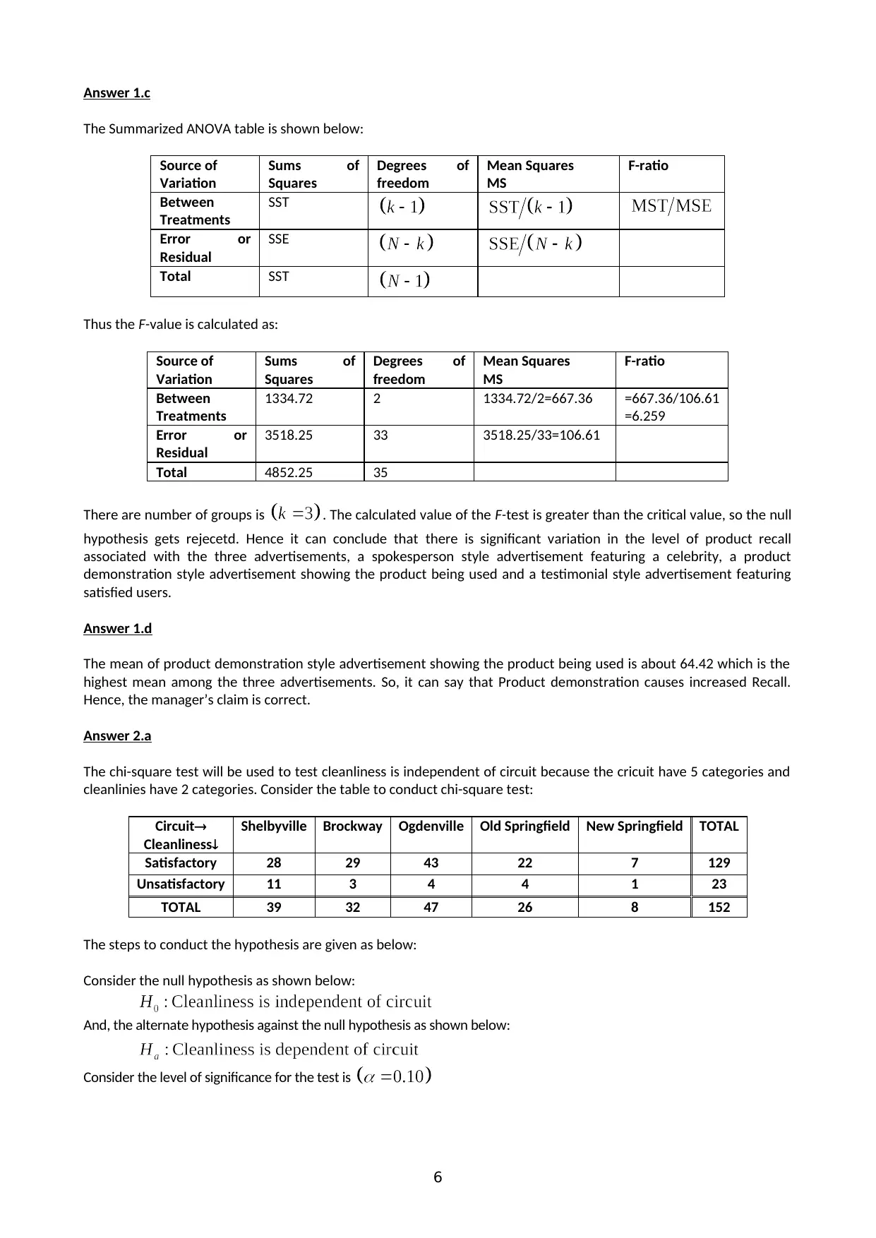
Answer 1.c
The Summarized ANOVA table is shown below:
Source of
Variation
Sums of
Squares
Degrees of
freedom
Mean Squares
MS
F-ratio
Between
Treatments
SST
Error or
Residual
SSE
Total SST
Thus the F-value is calculated as:
Source of
Variation
Sums of
Squares
Degrees of
freedom
Mean Squares
MS
F-ratio
Between
Treatments
1334.72 2 1334.72/2=667.36 =667.36/106.61
=6.259
Error or
Residual
3518.25 33 3518.25/33=106.61
Total 4852.25 35
There are number of groups is . The calculated value of the F-test is greater than the critical value, so the null
hypothesis gets rejecetd. Hence it can conclude that there is significant variation in the level of product recall
associated with the three advertisements, a spokesperson style advertisement featuring a celebrity, a product
demonstration style advertisement showing the product being used and a testimonial style advertisement featuring
satisfied users.
Answer 1.d
The mean of product demonstration style advertisement showing the product being used is about 64.42 which is the
highest mean among the three advertisements. So, it can say that Product demonstration causes increased Recall.
Hence, the manager’s claim is correct.
Answer 2.a
The chi-square test will be used to test cleanliness is independent of circuit because the cricuit have 5 categories and
cleanlinies have 2 categories. Consider the table to conduct chi-square test:
Circuit
Cleanliness
Shelbyville Brockway Ogdenville Old Springfield New Springfield TOTAL
Satisfactory 28 29 43 22 7 129
Unsatisfactory 11 3 4 4 1 23
TOTAL 39 32 47 26 8 152
The steps to conduct the hypothesis are given as below:
Consider the null hypothesis as shown below:
And, the alternate hypothesis against the null hypothesis as shown below:
Consider the level of significance for the test is
6
⊘ This is a preview!⊘
Do you want full access?
Subscribe today to unlock all pages.
Trusted by 1+ million students worldwide
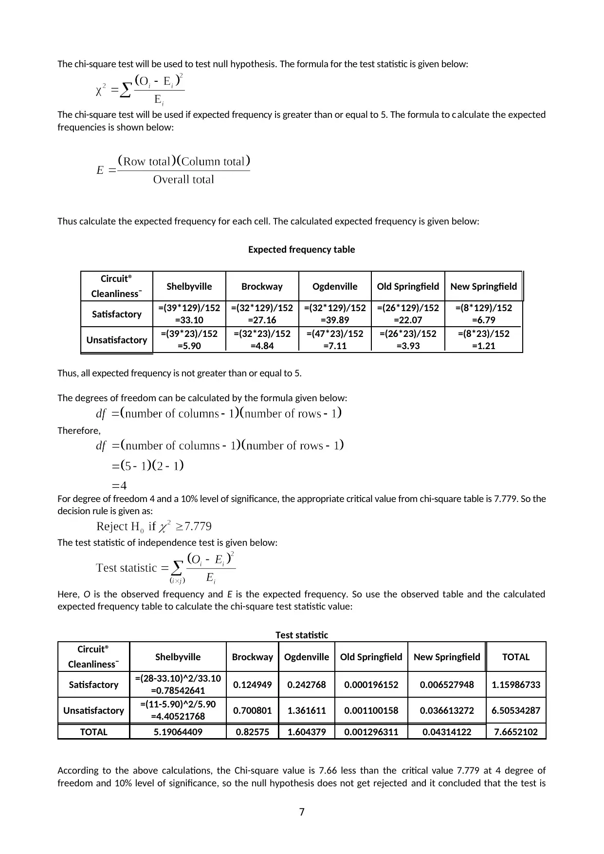
The chi-square test will be used to test null hypothesis. The formula for the test statistic is given below:
The chi-square test will be used if expected frequency is greater than or equal to 5. The formula to calculate the expected
frequencies is shown below:
Thus calculate the expected frequency for each cell. The calculated expected frequency is given below:
Expected frequency table
Circuit® Shelbyville Brockway Ogdenville Old Springfield New Springfield
Cleanliness¯
Satisfactory =(39*129)/152
=33.10
=(32*129)/152
=27.16
=(32*129)/152
=39.89
=(26*129)/152
=22.07
=(8*129)/152
=6.79
Unsatisfactory =(39*23)/152
=5.90
=(32*23)/152
=4.84
=(47*23)/152
=7.11
=(26*23)/152
=3.93
=(8*23)/152
=1.21
Thus, all expected frequency is not greater than or equal to 5.
The degrees of freedom can be calculated by the formula given below:
Therefore,
For degree of freedom 4 and a 10% level of significance, the appropriate critical value from chi-square table is 7.779. So the
decision rule is given as:
The test statistic of independence test is given below:
Here, O is the observed frequency and E is the expected frequency. So use the observed table and the calculated
expected frequency table to calculate the chi-square test statistic value:
Test statistic
Circuit® Shelbyville Brockway Ogdenville Old Springfield New Springfield TOTAL
Cleanliness¯
Satisfactory =(28-33.10)^2/33.10
=0.78542641 0.124949 0.242768 0.000196152 0.006527948 1.15986733
Unsatisfactory =(11-5.90)^2/5.90
=4.40521768 0.700801 1.361611 0.001100158 0.036613272 6.50534287
TOTAL 5.19064409 0.82575 1.604379 0.001296311 0.04314122 7.6652102
According to the above calculations, the Chi-square value is 7.66 less than the critical value 7.779 at 4 degree of
freedom and 10% level of significance, so the null hypothesis does not get rejected and it concluded that the test is
7
Paraphrase This Document
Need a fresh take? Get an instant paraphrase of this document with our AI Paraphraser
statistically significant at 10% level of significance. Hence, there is convincing evidence that cleanliness is independent
of circuit.
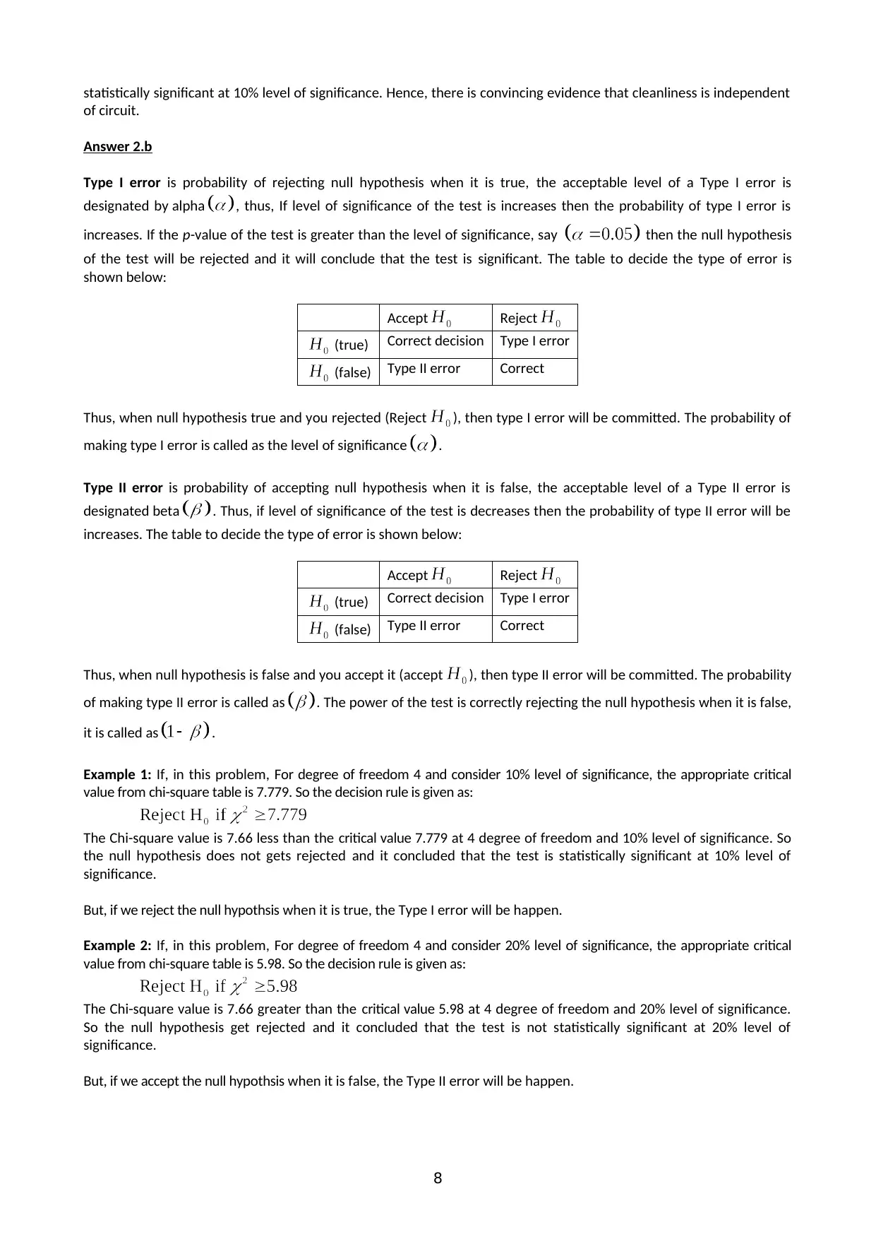
Answer 2.b
Type I error is probability of rejecting null hypothesis when it is true, the acceptable level of a Type I error is
designated by alpha , thus, If level of significance of the test is increases then the probability of type I error is
increases. If the p-value of the test is greater than the level of significance, say then the null hypothesis
of the test will be rejected and it will conclude that the test is significant. The table to decide the type of error is
shown below:
Accept Reject
(true) Correct decision Type I error
(false) Type II error Correct
Thus, when null hypothesis true and you rejected (Reject ), then type I error will be committed. The probability of
making type I error is called as the level of significance .
Type II error is probability of accepting null hypothesis when it is false, the acceptable level of a Type II error is
designated beta . Thus, if level of significance of the test is decreases then the probability of type II error will be
increases. The table to decide the type of error is shown below:
Accept Reject
(true) Correct decision Type I error
(false) Type II error Correct
Thus, when null hypothesis is false and you accept it (accept ), then type II error will be committed. The probability
of making type II error is called as . The power of the test is correctly rejecting the null hypothesis when it is false,
it is called as .
Example 1: If, in this problem, For degree of freedom 4 and consider 10% level of significance, the appropriate critical
value from chi-square table is 7.779. So the decision rule is given as:
The Chi-square value is 7.66 less than the critical value 7.779 at 4 degree of freedom and 10% level of significance. So
the null hypothesis does not gets rejected and it concluded that the test is statistically significant at 10% level of
significance.
But, if we reject the null hypothsis when it is true, the Type I error will be happen.
Example 2: If, in this problem, For degree of freedom 4 and consider 20% level of significance, the appropriate critical
value from chi-square table is 5.98. So the decision rule is given as:
The Chi-square value is 7.66 greater than the critical value 5.98 at 4 degree of freedom and 20% level of significance.
So the null hypothesis get rejected and it concluded that the test is not statistically significant at 20% level of
significance.
But, if we accept the null hypothsis when it is false, the Type II error will be happen.
8
of circuit.
Answer 2.b
Type I error is probability of rejecting null hypothesis when it is true, the acceptable level of a Type I error is
designated by alpha , thus, If level of significance of the test is increases then the probability of type I error is
increases. If the p-value of the test is greater than the level of significance, say then the null hypothesis
of the test will be rejected and it will conclude that the test is significant. The table to decide the type of error is
shown below:
Accept Reject
(true) Correct decision Type I error
(false) Type II error Correct
Thus, when null hypothesis true and you rejected (Reject ), then type I error will be committed. The probability of
making type I error is called as the level of significance .
Type II error is probability of accepting null hypothesis when it is false, the acceptable level of a Type II error is
designated beta . Thus, if level of significance of the test is decreases then the probability of type II error will be
increases. The table to decide the type of error is shown below:
Accept Reject
(true) Correct decision Type I error
(false) Type II error Correct
Thus, when null hypothesis is false and you accept it (accept ), then type II error will be committed. The probability
of making type II error is called as . The power of the test is correctly rejecting the null hypothesis when it is false,
it is called as .
Example 1: If, in this problem, For degree of freedom 4 and consider 10% level of significance, the appropriate critical
value from chi-square table is 7.779. So the decision rule is given as:
The Chi-square value is 7.66 less than the critical value 7.779 at 4 degree of freedom and 10% level of significance. So
the null hypothesis does not gets rejected and it concluded that the test is statistically significant at 10% level of
significance.
But, if we reject the null hypothsis when it is true, the Type I error will be happen.
Example 2: If, in this problem, For degree of freedom 4 and consider 20% level of significance, the appropriate critical
value from chi-square table is 5.98. So the decision rule is given as:
The Chi-square value is 7.66 greater than the critical value 5.98 at 4 degree of freedom and 20% level of significance.
So the null hypothesis get rejected and it concluded that the test is not statistically significant at 20% level of
significance.
But, if we accept the null hypothsis when it is false, the Type II error will be happen.
8
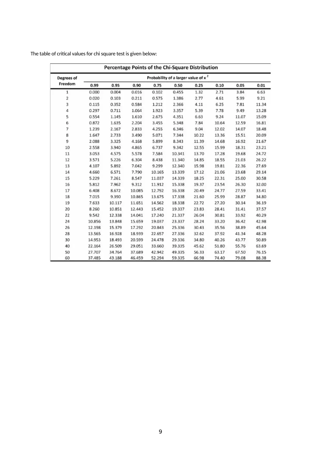
The table of critical values for chi square test is given below:
9
9
⊘ This is a preview!⊘
Do you want full access?
Subscribe today to unlock all pages.
Trusted by 1+ million students worldwide
1 out of 9
Your All-in-One AI-Powered Toolkit for Academic Success.
+13062052269
info@desklib.com
Available 24*7 on WhatsApp / Email
![[object Object]](/_next/static/media/star-bottom.7253800d.svg)
Unlock your academic potential
Copyright © 2020–2026 A2Z Services. All Rights Reserved. Developed and managed by ZUCOL.