Quantitative Methods with Economics (MAT10706) Project Analysis

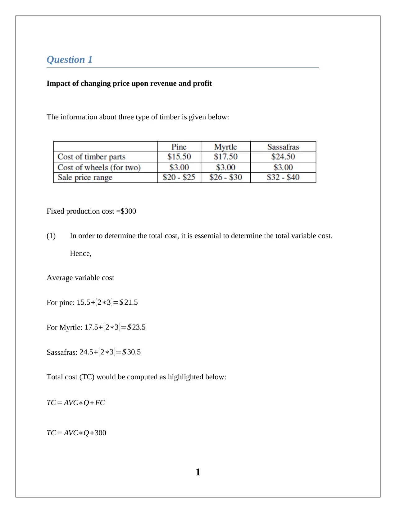
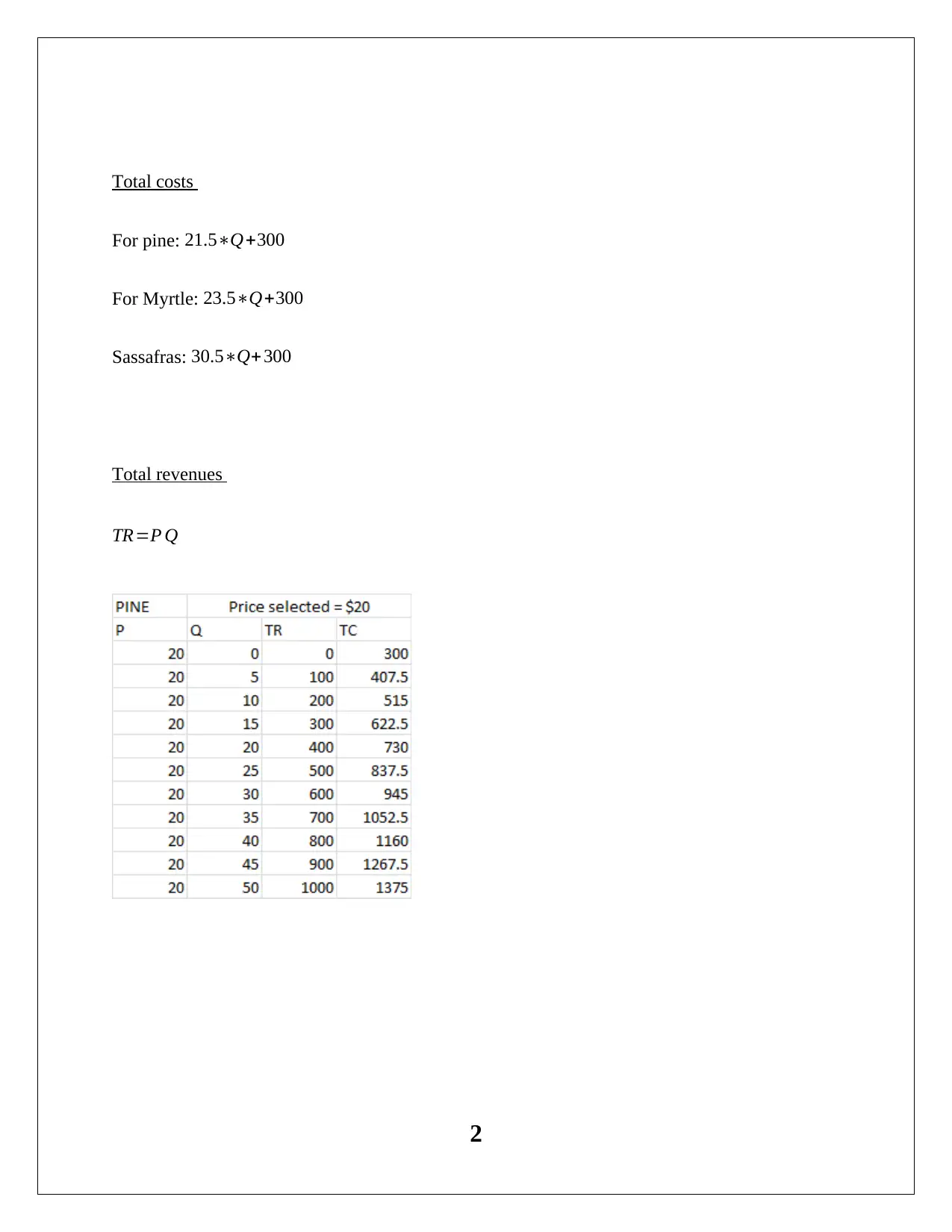
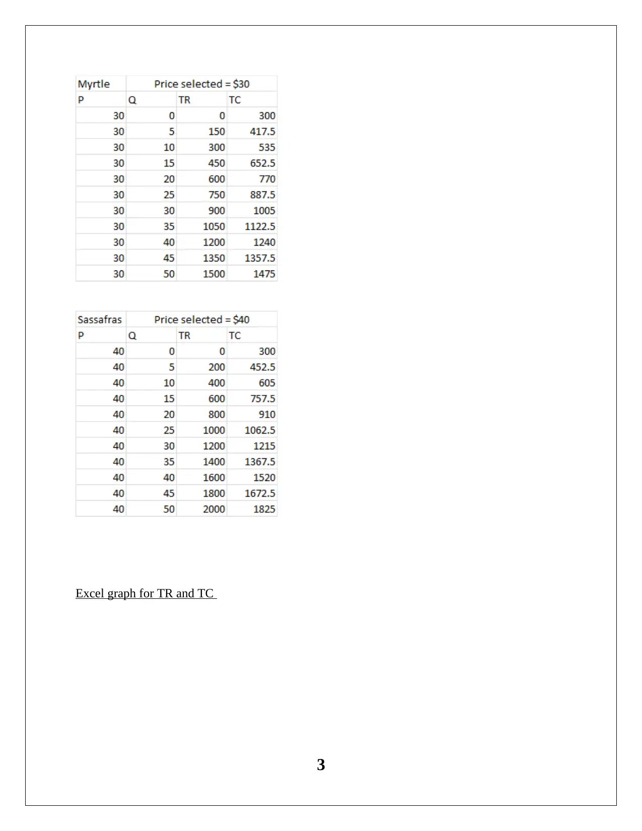
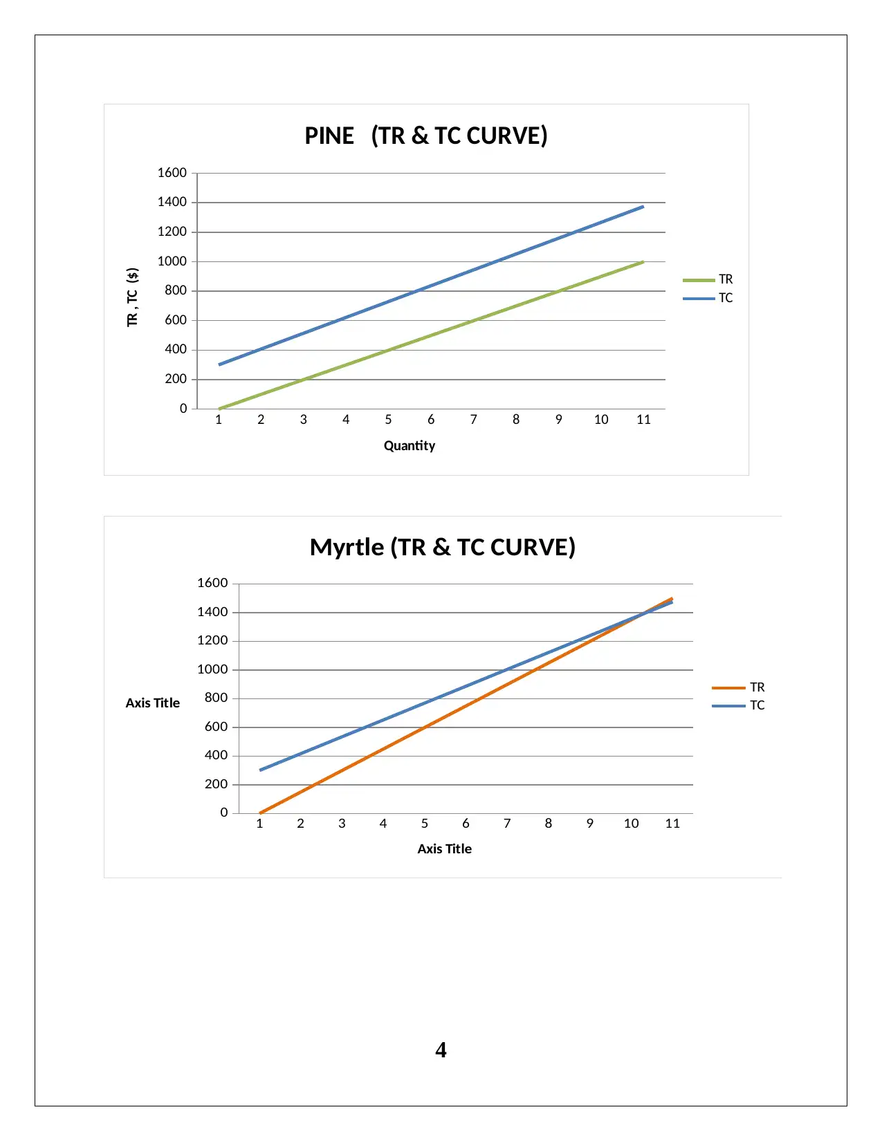
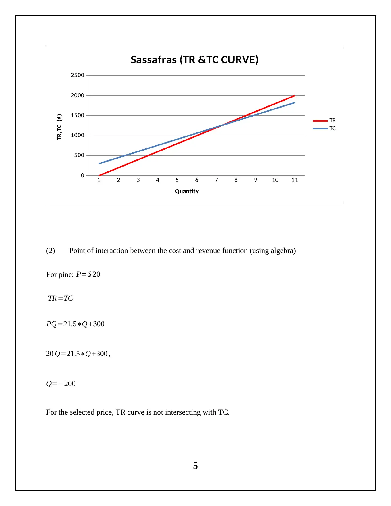
This project analyzes the impact of price changes on revenue and profit, examining three types of timber and their production costs, revenues, and break-even points. The first part of the project explores the relationship between price, revenue, and profit for different timber products, calculating total costs, revenues, and identifying break-even points using algebraic methods and Excel graphs. The project determines the point where total cost equals total revenue. The second part investigates the impact of a price discount on revenue, analyzing supply and demand equations, calculating equilibrium prices and quantities before and after a price reduction, and assessing the price elasticity of demand. The analysis concludes that a price decrease is not recommended, as the resulting increase in quantity is insufficient to offset the reduced revenue per customer. The project highlights the importance of break-even analysis and understanding price elasticity in making informed business decisions.

MAT10706 QUANTITATIVE METHODS WITH ECONOMICS
PROJECT ASSIGNMENT
Student
[Pick the date]

Question 1
Impact of changing price upon revenue and profit
The information about three type of timber is given below:
Fixed production cost =$300
(1) In order to determine the total cost, it is essential to determine the total variable cost.
Hence,
Average variable cost
For pine: 15.5+ ( 2∗3 )=$ 21.5
For Myrtle: 17.5+ ( 2∗3 )=$ 23.5
Sassafras: 24.5+ ( 2∗3 ) =$ 30.5
Total cost (TC) would be computed as highlighted below:
TC= AVC∗Q+FC
TC= AVC∗Q+300
1

Total costs
For pine: 21.5∗Q+300
For Myrtle: 23.5∗Q+300
Sassafras: 30.5∗Q+ 300
Total revenues
TR=P Q
2

Excel graph for TR and TC
3

1 2 3 4 5 6 7 8 9 10 11
0
200
400
600
800
1000
1200
1400
1600
PINE (TR & TC CURVE)
TR
TC
Quantity
TR , TC ($)
1 2 3 4 5 6 7 8 9 10 11
0
200
400
600
800
1000
1200
1400
1600
Myrtle (TR & TC CURVE)
TR
TC
Axis Title
Axis Title
4

1 2 3 4 5 6 7 8 9 10 11
0
500
1000
1500
2000
2500
Sassafras (TR &TC CURVE)
TR
TC
Quantity
TR, TC ($)
(2) Point of interaction between the cost and revenue function (using algebra)
For pine: P=$ 20
TR=TC
PQ=21.5∗Q+300
20 Q=21.5∗Q+300 ,
Q=−200
For the selected price, TR curve is not intersecting with TC.
5

For Myrtle: P=$ 30
30 Q=23.5∗Q+300
Q=46.15
Intersection point between TR and TC is at Q=46.15.
Sassafras: P=$ 40
40 Q=30.5∗Q+300
Q=31.58
Intersection point between TR and TC is at Q=31.58.
(3) Profit function and break-even point
Profit ¿ TR−TC
At break-even point, TR = TC and so, TR and T would intersect.
For pine:
Profit=TR−TC
6

¿ PQ−21.5∗Q−300=−1.5 Q−300
No breakeven present because TR and TC curves are not intersecting.
For Myrtle:
Profit=30 Q−23.5∗Q−300=6.5 Q−300
Intersection point between TR and TC is 46.15 46 which the breakeven quantity is 46.
Sassafras:
Profit=40Q−30.5∗Q−300=9.5Q−300
Intersection point between TR and TC is 31.58 32 which the breakeven quantity is 32.
(4) Summary
a) The intersection of total cost (TC) and total revenue (TR) represents the point at which the
two values would be equal. Since at this point, the total cost would be equal to the total
revenue; hence no profit or loss would be incurred. This is referred to as break-even point.
The existence of this point implies that the company can earn profits if the underlying
quantity is greater than the break even quantity. Absence of intersection point would imply
7

that breakeven point does not exist which implies that the given product line would be loss
making and hence not sustainable.
b) It is easiest to make profit on Sassafras since the break-even for this insect is achieved at the
lowest quantity and hence any quantity greater than the break even quantity of 31.58 would
lead to profit generation. Next in line, would be the Myrtle insect for which break even
quantity is slightly higher at 46.15 and hence only when 47 insects of this model are sold
would the company make profits. However, the company would not make any profit on Pine
insect irrespective of the quantity sold.
c) It is assumed that the fixed costs does not alter and also unit variable cost does not change
with the increase or decrease in the units produced. Also, the price charged tends to remain
constant.
8

Question 2
Impact of price discount on revenue
Supply and demand equations are given below:
Demand equation p=150−10 aq
Supply equation p=0.00001q2+2bq +20
Where,
q=number of customers ( ¿ hundreds per year )
p= price of dinner (dollars)
a , b=coefficients
(1) Two random numbers for a and b between 0.1 and 0.9 is selected as
a 0.25305
6
b 0.13103
1
9

(2) Equilibrium price and quantity would be determined as
150−10 aq=0.00001q2+ 2bq +20
150− ( 10∗0.253 ) q=0.0000 1 q2 +(2∗0.131) q+20
150−2.53 q=0.00001 q2+0.262q+20
0.0000 1 q2 +2.792 q−130=0
q=46.55 ,−279246.5
Quantity cannot be negative and hence, equilibrium quantity would be 46.5.
Equilibrium price p=150−10 aq
¿ 150− (10∗0.253∗46.5 )=$ 32.35
(3) Updated demand equation by considering $15 price decrease.
Now, p= p−15
Demand equation p=150−10 aq
p−15=150−10 aq
p=165−10∗0.253 q
10

p=165−2.53 q (Updated demand eq .)
(4) New equilibrium price and quantity with the help of algebra is given below:
165−2.53 q=0.00001q2+2bq +20
165−2.53 q=0.00001 q2+0.262q+20
0.0000 1 q2 +2.792 q−145=0
q=51.92 ,−279251
Quantity cannot be negative and hence, equilibrium quantity would be 51.92.
Equilibrium price ¿ p=165− ( 2.53∗51.92 ) =$ 33.64
(5) Demand and supply curve is given below:
11

0 20 40 60 80 100 120 140 160
0
10
20
30
40
50
60
70
Demand and Supply Curve
Quantity Demanded Quantity Supplied Quantiy Demanded(new)
Quantity
Price ($)
(6) Summary table
Before price
reduction
After price
reduction
Difference
Equilibrium quantity 46.55 51.92 5.37
Equilibrium price: consumer pays 32.35 33.64 1.29
Equilibrium price: restaurant would charge
without any price reduction
32.35 32.35 0.00
Revenue restaurant would receive without any
price reduction
1505.89 1679.6 173.72
12