Alternative Assessment: Quantitative Methods for Business Report
VerifiedAdded on 2023/01/11
|16
|4495
|81
Report
AI Summary
This report addresses various quantitative methods relevant to business analysis and decision-making. It begins with an analysis of access time in a computer disc system, calculating mean and standard deviation to understand data distribution. Different sampling methods, including simple random sampling, quota sampling, cluster sampling, and systematic sampling, are illustrated with practical examples. The report then delves into regression analysis, explaining the meaning of regression coefficients and applying them to select the best car model for business expansion in a new region, considering increased travel distances. Finally, it covers probability calculations in different scenarios involving John, Albert, and Chris, and also for box A and box B. The report utilizes formulas, calculations, and interpretations to provide a comprehensive understanding of the concepts.

Alternative questions
Paraphrase This Document
Need a fresh take? Get an instant paraphrase of this document with our AI Paraphraser
Table of Contents
Table of Contents.............................................................................................................................2
INTRODUCTION...........................................................................................................................1
QUESTION 1..................................................................................................................................1
a. Analysis of the access time to a computer disc system...........................................................1
b. Illustration of different types of sampling methods along with practical examples................3
c. Cumulative frequency distribution from the data and using seven class intervals..................5
QUESTION 2..................................................................................................................................6
a. Meaning of four regression coefficients for the provided data................................................6
b. Selecting on best type of car model to expand business in a new region................................7
c. Calculation of running costs for 5 of the cars when the costs will be increased up to 10%....9
QUESTION 3................................................................................................................................10
a. Calculation of probability for John, Albert and Chris...........................................................10
(b) Calculating the probability for box A and box B.................................................................12
CONCLUSION..............................................................................................................................13
REFERENCES..............................................................................................................................14
INTRODUCTION
Quantitative methods are considered as the main part of statistics which are used by
researchers for the purpose of getting accurate outcomes for the research questions (Aidara,
2018). There are various types of them which are forecasting, data mining, project management
etc. Purpose of this assignment is to develop understanding of various types of quantitative
methods which could be used to find appropriate solutions for the research problems. For the
purpose of completing this report three questions which are selected are one, two and three. For
the completion of the project, the topics which will be covered in it are different types of
sampling, regression, mean, standard deviation, probability etc.
QUESTION 1
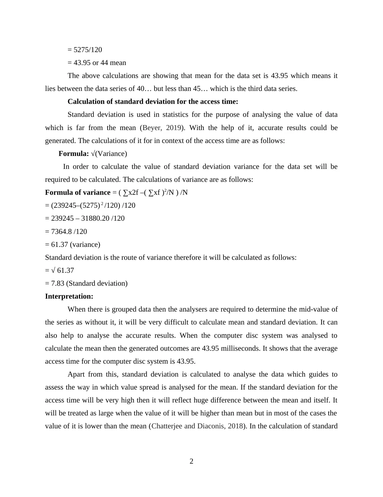
a. Analysis of the access time to a computer disc system
By analysing the scenario, it has been determined thar access time for the computer disc
system is assessed for 1290 time. In order to analyse the access time further standard deviation
and mean for the same is calculated. All the calculations are as follows:
Calculation of mean for the access time:
Access time
(milliseconds)
Frequency
(f)
Mid-point
(x) f x x2 f
30… but less than 35… 17… 32… 544… 17408…
35… but less than 40… 24… 37… 888… 32856…
40… but less than 45… 19… 42… 798… 33516…
45… but less than 50… 28… 47… 1316… 61852…
50… but less than 55… 19… 52… 988… 51376…
55… but less than 60… 13… 57… 741… 42237…
Total N = 120… 5275… 239245…
Mean can be defined as the average value of the data set. In order to calculate it the total
values in the data set are divided by the total of the values. Sometime different formulas for the
calculation of it are applied (Akyüz and Abu-Shawiesh, 2020). As in the above table, it is
calculated by dividing the total frequencies with the total of fx which is multiplication of
frequency and mid-point. The calculation of the same is as follows:
Formula: Total value of fx / total number of frequencies
1
Quantitative methods are considered as the main part of statistics which are used by
researchers for the purpose of getting accurate outcomes for the research questions (Aidara,
2018). There are various types of them which are forecasting, data mining, project management
etc. Purpose of this assignment is to develop understanding of various types of quantitative
methods which could be used to find appropriate solutions for the research problems. For the
purpose of completing this report three questions which are selected are one, two and three. For
the completion of the project, the topics which will be covered in it are different types of
sampling, regression, mean, standard deviation, probability etc.
QUESTION 1
a. Analysis of the access time to a computer disc system
By analysing the scenario, it has been determined thar access time for the computer disc
system is assessed for 1290 time. In order to analyse the access time further standard deviation
and mean for the same is calculated. All the calculations are as follows:
Calculation of mean for the access time:
Access time
(milliseconds)
Frequency
(f)
Mid-point
(x) f x x2 f
30… but less than 35… 17… 32… 544… 17408…
35… but less than 40… 24… 37… 888… 32856…
40… but less than 45… 19… 42… 798… 33516…
45… but less than 50… 28… 47… 1316… 61852…
50… but less than 55… 19… 52… 988… 51376…
55… but less than 60… 13… 57… 741… 42237…
Total N = 120… 5275… 239245…
Mean can be defined as the average value of the data set. In order to calculate it the total
values in the data set are divided by the total of the values. Sometime different formulas for the
calculation of it are applied (Akyüz and Abu-Shawiesh, 2020). As in the above table, it is
calculated by dividing the total frequencies with the total of fx which is multiplication of
frequency and mid-point. The calculation of the same is as follows:
Formula: Total value of fx / total number of frequencies
1
⊘ This is a preview!⊘
Do you want full access?
Subscribe today to unlock all pages.
Trusted by 1+ million students worldwide
= 5275/120
= 43.95 or 44 mean
The above calculations are showing that mean for the data set is 43.95 which means it
lies between the data series of 40… but less than 45… which is the third data series.
Calculation of standard deviation for the access time:
Standard deviation is used in statistics for the purpose of analysing the value of data
which is far from the mean (Beyer, 2019). With the help of it, accurate results could be
generated. The calculations of it for in context of the access time are as follows:
Formula: √(Variance)
In order to calculate the value of standard deviation variance for the data set will be
required to be calculated. The calculations of variance are as follows:
Formula of variance = ( ∑x2f –( ∑xf )2/N ) /N
= (239245–(5275) 2 /120) /120
= 239245 – 31880.20 /120
= 7364.8 /120
= 61.37 (variance)
Standard deviation is the route of variance therefore it will be calculated as follows:
= √ 61.37
= 7.83 (Standard deviation)
Interpretation:
When there is grouped data then the analysers are required to determine the mid-value of
the series as without it, it will be very difficult to calculate mean and standard deviation. It can
also help to analyse the accurate results. When the computer disc system was analysed to
calculate the mean then the generated outcomes are 43.95 milliseconds. It shows that the average
access time for the computer disc system is 43.95.
Apart from this, standard deviation is calculated to analyse the data which guides to
assess the way in which value spread is analysed for the mean. If the standard deviation for the
access time will be very high then it will reflect huge difference between the mean and itself. It
will be treated as large when the value of it will be higher than mean but in most of the cases the
value of it is lower than the mean (Chatterjee and Diaconis, 2018). In the calculation of standard
2
Paraphrase This Document
Need a fresh take? Get an instant paraphrase of this document with our AI Paraphraser
deviation for the access time the results generated are showing that the SD for the data series is
7.83 milliseconds.
As a conclusion it could be said that the average access time for the computer disc system
is 43.95 milliseconds which may vary +/- up to 7.83 milliseconds.
b. Illustration of different types of sampling methods along with practical examples
Sampling can be defined as a small portion of a large data which is selected for the purpose
of generating results or reaching to the conclusions. There are various types of it which are
described below along with specific examples of the same:
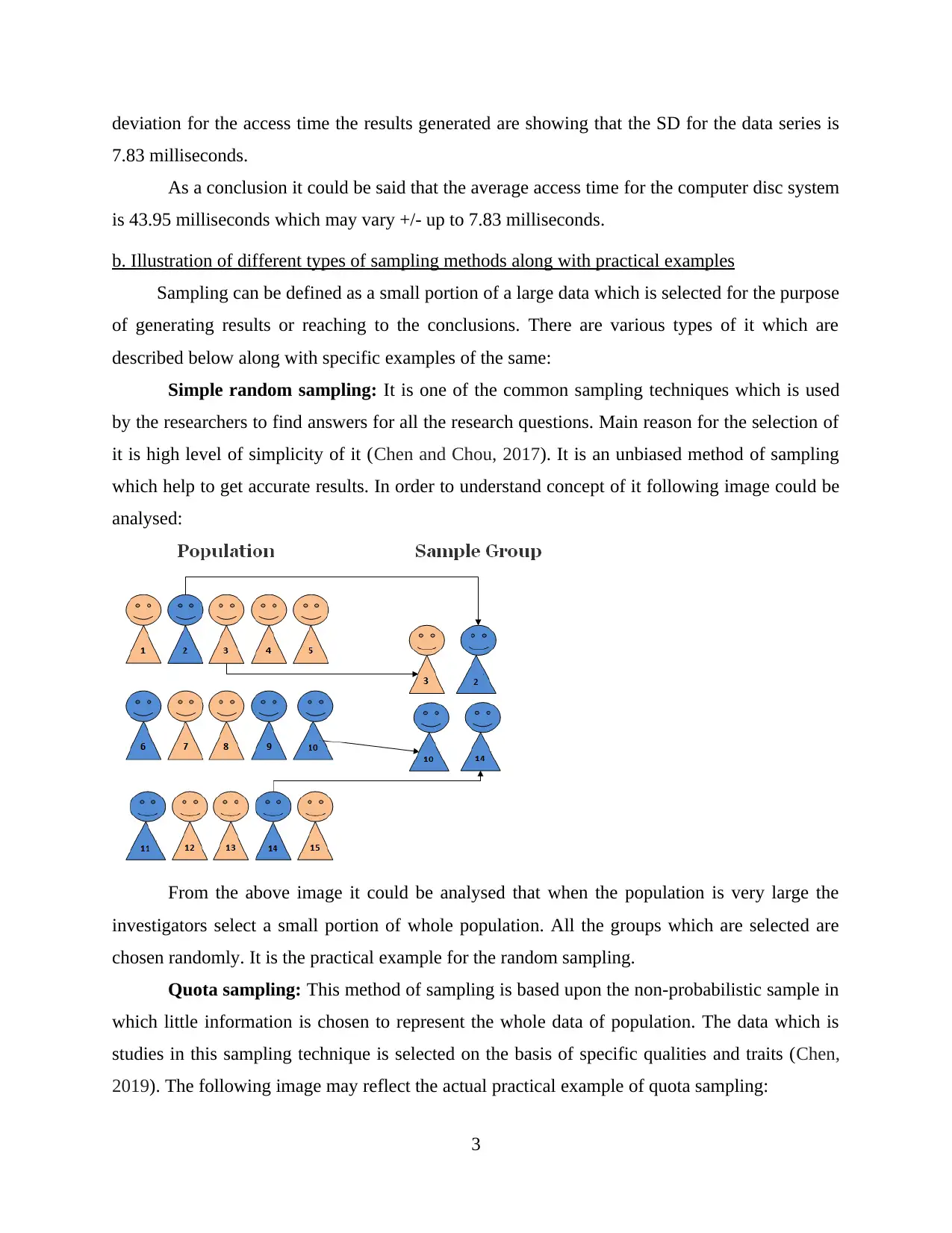
Simple random sampling: It is one of the common sampling techniques which is used
by the researchers to find answers for all the research questions. Main reason for the selection of
it is high level of simplicity of it (Chen and Chou, 2017). It is an unbiased method of sampling
which help to get accurate results. In order to understand concept of it following image could be
analysed:
From the above image it could be analysed that when the population is very large the
investigators select a small portion of whole population. All the groups which are selected are
chosen randomly. It is the practical example for the random sampling.
Quota sampling: This method of sampling is based upon the non-probabilistic sample in
which little information is chosen to represent the whole data of population. The data which is
studies in this sampling technique is selected on the basis of specific qualities and traits (Chen,
2019). The following image may reflect the actual practical example of quota sampling:
3
7.83 milliseconds.
As a conclusion it could be said that the average access time for the computer disc system
is 43.95 milliseconds which may vary +/- up to 7.83 milliseconds.
b. Illustration of different types of sampling methods along with practical examples
Sampling can be defined as a small portion of a large data which is selected for the purpose
of generating results or reaching to the conclusions. There are various types of it which are
described below along with specific examples of the same:
Simple random sampling: It is one of the common sampling techniques which is used
by the researchers to find answers for all the research questions. Main reason for the selection of
it is high level of simplicity of it (Chen and Chou, 2017). It is an unbiased method of sampling
which help to get accurate results. In order to understand concept of it following image could be
analysed:
From the above image it could be analysed that when the population is very large the
investigators select a small portion of whole population. All the groups which are selected are
chosen randomly. It is the practical example for the random sampling.
Quota sampling: This method of sampling is based upon the non-probabilistic sample in
which little information is chosen to represent the whole data of population. The data which is
studies in this sampling technique is selected on the basis of specific qualities and traits (Chen,
2019). The following image may reflect the actual practical example of quota sampling:
3
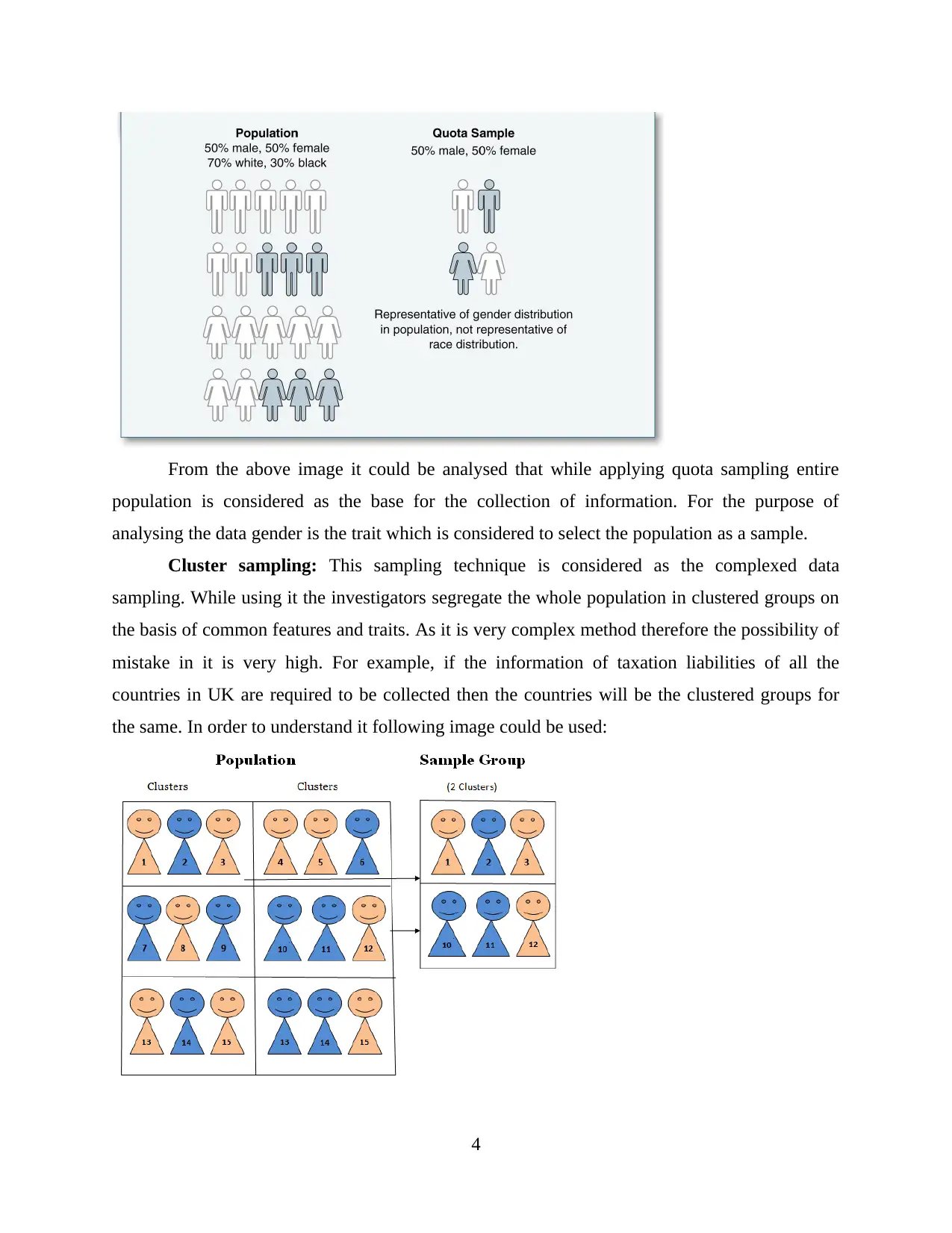
From the above image it could be analysed that while applying quota sampling entire
population is considered as the base for the collection of information. For the purpose of
analysing the data gender is the trait which is considered to select the population as a sample.
Cluster sampling: This sampling technique is considered as the complexed data
sampling. While using it the investigators segregate the whole population in clustered groups on
the basis of common features and traits. As it is very complex method therefore the possibility of
mistake in it is very high. For example, if the information of taxation liabilities of all the
countries in UK are required to be collected then the countries will be the clustered groups for
the same. In order to understand it following image could be used:
4
⊘ This is a preview!⊘
Do you want full access?
Subscribe today to unlock all pages.
Trusted by 1+ million students worldwide
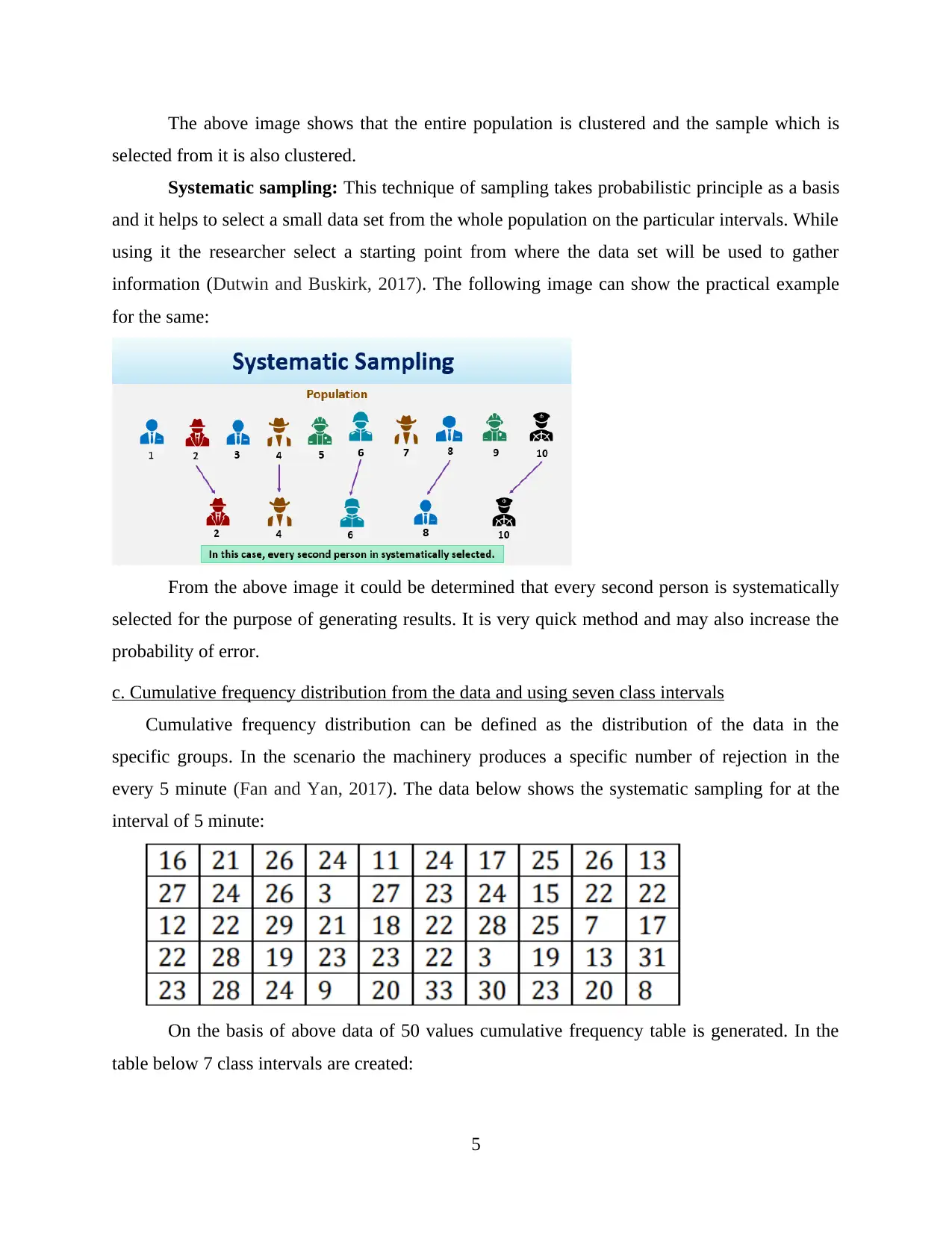
The above image shows that the entire population is clustered and the sample which is
selected from it is also clustered.
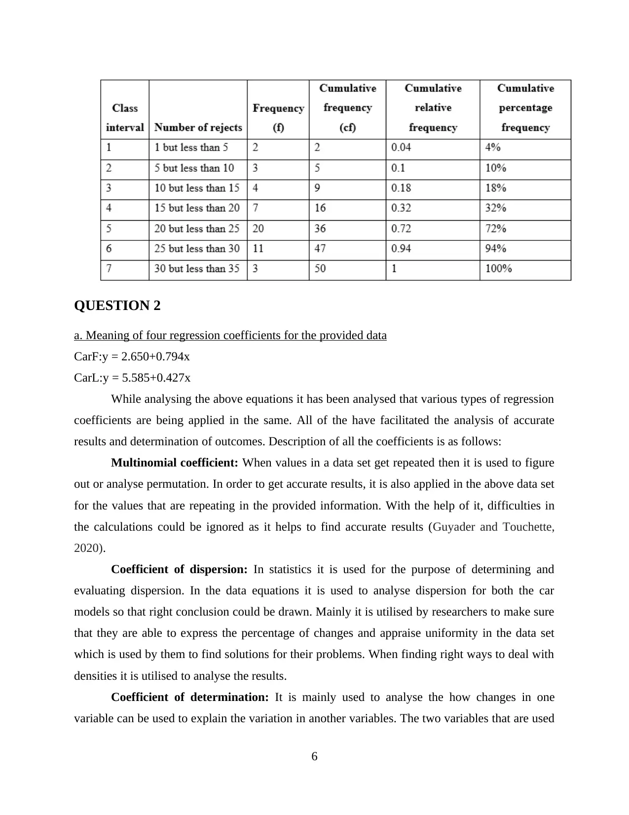
Systematic sampling: This technique of sampling takes probabilistic principle as a basis
and it helps to select a small data set from the whole population on the particular intervals. While
using it the researcher select a starting point from where the data set will be used to gather
information (Dutwin and Buskirk, 2017). The following image can show the practical example
for the same:
From the above image it could be determined that every second person is systematically
selected for the purpose of generating results. It is very quick method and may also increase the
probability of error.
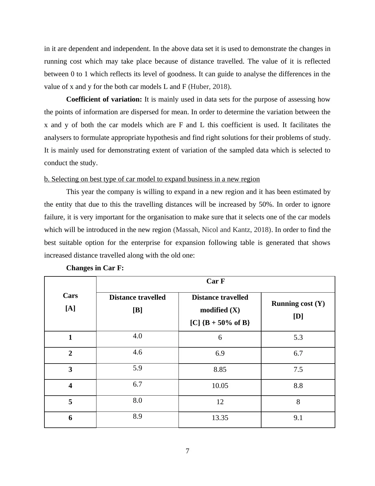
c. Cumulative frequency distribution from the data and using seven class intervals
Cumulative frequency distribution can be defined as the distribution of the data in the
specific groups. In the scenario the machinery produces a specific number of rejection in the
every 5 minute (Fan and Yan, 2017). The data below shows the systematic sampling for at the
interval of 5 minute:
On the basis of above data of 50 values cumulative frequency table is generated. In the
table below 7 class intervals are created:
5
selected from it is also clustered.
Systematic sampling: This technique of sampling takes probabilistic principle as a basis
and it helps to select a small data set from the whole population on the particular intervals. While
using it the researcher select a starting point from where the data set will be used to gather
information (Dutwin and Buskirk, 2017). The following image can show the practical example
for the same:
From the above image it could be determined that every second person is systematically
selected for the purpose of generating results. It is very quick method and may also increase the
probability of error.
c. Cumulative frequency distribution from the data and using seven class intervals
Cumulative frequency distribution can be defined as the distribution of the data in the
specific groups. In the scenario the machinery produces a specific number of rejection in the
every 5 minute (Fan and Yan, 2017). The data below shows the systematic sampling for at the
interval of 5 minute:
On the basis of above data of 50 values cumulative frequency table is generated. In the
table below 7 class intervals are created:
5
Paraphrase This Document
Need a fresh take? Get an instant paraphrase of this document with our AI Paraphraser
QUESTION 2
a. Meaning of four regression coefficients for the provided data
CarF:y = 2.650+0.794x
CarL:y = 5.585+0.427x
While analysing the above equations it has been analysed that various types of regression
coefficients are being applied in the same. All of the have facilitated the analysis of accurate
results and determination of outcomes. Description of all the coefficients is as follows:
Multinomial coefficient: When values in a data set get repeated then it is used to figure
out or analyse permutation. In order to get accurate results, it is also applied in the above data set
for the values that are repeating in the provided information. With the help of it, difficulties in
the calculations could be ignored as it helps to find accurate results (Guyader and Touchette,
2020).
Coefficient of dispersion: In statistics it is used for the purpose of determining and
evaluating dispersion. In the data equations it is used to analyse dispersion for both the car
models so that right conclusion could be drawn. Mainly it is utilised by researchers to make sure
that they are able to express the percentage of changes and appraise uniformity in the data set
which is used by them to find solutions for their problems. When finding right ways to deal with
densities it is utilised to analyse the results.
Coefficient of determination: It is mainly used to analyse the how changes in one
variable can be used to explain the variation in another variables. The two variables that are used
6
in it are dependent and independent. In the above data set it is used to demonstrate the changes in
running cost which may take place because of distance travelled. The value of it is reflected
between 0 to 1 which reflects its level of goodness. It can guide to analyse the differences in the
value of x and y for the both car models L and F (Huber, 2018).
Coefficient of variation: It is mainly used in data sets for the purpose of assessing how
the points of information are dispersed for mean. In order to determine the variation between the
x and y of both the car models which are F and L this coefficient is used. It facilitates the
analysers to formulate appropriate hypothesis and find right solutions for their problems of study.
It is mainly used for demonstrating extent of variation of the sampled data which is selected to
conduct the study.
b. Selecting on best type of car model to expand business in a new region
This year the company is willing to expand in a new region and it has been estimated by
the entity that due to this the travelling distances will be increased by 50%. In order to ignore
failure, it is very important for the organisation to make sure that it selects one of the car models
which will be introduced in the new region (Massah, Nicol and Kantz, 2018). In order to find the
best suitable option for the enterprise for expansion following table is generated that shows
increased distance travelled along with the old one:
Changes in Car F:
Cars
[A]
Car F
Distance travelled
[B]
Distance travelled
modified (X)
[C] {B + 50% of B}
Running cost (Y)
[D]
1 4.0 6 5.3
2 4.6 6.9 6.7
3 5.9 8.85 7.5
4 6.7 10.05 8.8
5 8.0 12 8
6 8.9 13.35 9.1
7
⊘ This is a preview!⊘
Do you want full access?
Subscribe today to unlock all pages.
Trusted by 1+ million students worldwide
7 8.9 13.35 10.5
8 10.1 15.15 10
9 10.8 16.2 11.7
10 12.1 18.15 12.4
Mean 8 12 9
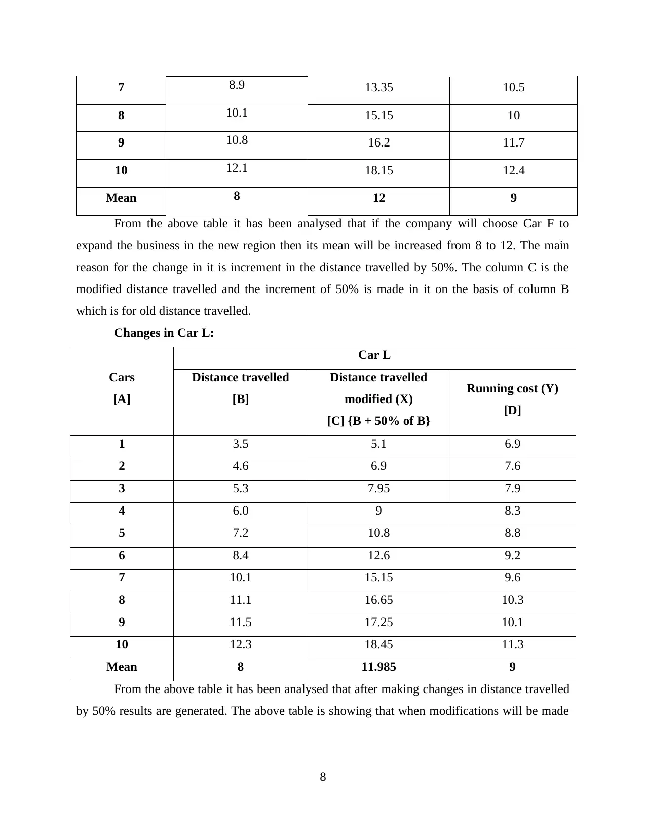
From the above table it has been analysed that if the company will choose Car F to
expand the business in the new region then its mean will be increased from 8 to 12. The main
reason for the change in it is increment in the distance travelled by 50%. The column C is the
modified distance travelled and the increment of 50% is made in it on the basis of column B
which is for old distance travelled.
Changes in Car L:
Cars
[A]
Car L
Distance travelled
[B]
Distance travelled
modified (X)
[C] {B + 50% of B}
Running cost (Y)
[D]
1 3.5 5.1 6.9
2 4.6 6.9 7.6
3 5.3 7.95 7.9
4 6.0 9 8.3
5 7.2 10.8 8.8
6 8.4 12.6 9.2
7 10.1 15.15 9.6
8 11.1 16.65 10.3
9 11.5 17.25 10.1
10 12.3 18.45 11.3
Mean 8 11.985 9
From the above table it has been analysed that after making changes in distance travelled
by 50% results are generated. The above table is showing that when modifications will be made
8
8 10.1 15.15 10
9 10.8 16.2 11.7
10 12.1 18.15 12.4
Mean 8 12 9
From the above table it has been analysed that if the company will choose Car F to
expand the business in the new region then its mean will be increased from 8 to 12. The main
reason for the change in it is increment in the distance travelled by 50%. The column C is the
modified distance travelled and the increment of 50% is made in it on the basis of column B
which is for old distance travelled.
Changes in Car L:
Cars
[A]
Car L
Distance travelled
[B]
Distance travelled
modified (X)
[C] {B + 50% of B}
Running cost (Y)
[D]
1 3.5 5.1 6.9
2 4.6 6.9 7.6
3 5.3 7.95 7.9
4 6.0 9 8.3
5 7.2 10.8 8.8
6 8.4 12.6 9.2
7 10.1 15.15 9.6
8 11.1 16.65 10.3
9 11.5 17.25 10.1
10 12.3 18.45 11.3
Mean 8 11.985 9
From the above table it has been analysed that after making changes in distance travelled
by 50% results are generated. The above table is showing that when modifications will be made
8
Paraphrase This Document
Need a fresh take? Get an instant paraphrase of this document with our AI Paraphraser
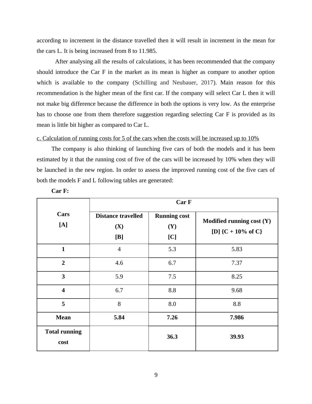
according to increment in the distance travelled then it will result in increment in the mean for
the cars L. It is being increased from 8 to 11.985.
After analysing all the results of calculations, it has been recommended that the company
should introduce the Car F in the market as its mean is higher as compare to another option
which is available to the company (Schilling and Neubauer, 2017). Main reason for this
recommendation is the higher mean of the first car. If the company will select Car L then it will
not make big difference because the difference in both the options is very low. As the enterprise
has to choose one from them therefore suggestion regarding selecting Car F is provided as its
mean is little bit higher as compared to Car L.
c. Calculation of running costs for 5 of the cars when the costs will be increased up to 10%
The company is also thinking of launching five cars of both the models and it has been
estimated by it that the running cost of five of the cars will be increased by 10% when they will
be launched in the new region. In order to assess the improved running cost of the five cars of
both the models F and L following tables are generated:
Car F:
Cars
[A]
Car F
Distance travelled
(X)
[B]
Running cost
(Y)
[C]
Modified running cost (Y)
[D] {C + 10% of C}
1 4 5.3 5.83
2 4.6 6.7 7.37
3 5.9 7.5 8.25
4 6.7 8.8 9.68
5 8 8.0 8.8
Mean 5.84 7.26 7.986
Total running
cost 36.3 39.93
9
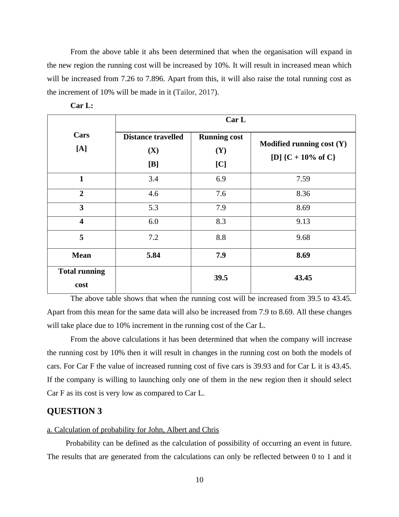
From the above table it ahs been determined that when the organisation will expand in
the new region the running cost will be increased by 10%. It will result in increased mean which
will be increased from 7.26 to 7.896. Apart from this, it will also raise the total running cost as
the increment of 10% will be made in it (Tailor, 2017).
Car L:
Cars
[A]
Car L
Distance travelled
(X)
[B]
Running cost
(Y)
[C]
Modified running cost (Y)
[D] {C + 10% of C}
1 3.4 6.9 7.59
2 4.6 7.6 8.36
3 5.3 7.9 8.69
4 6.0 8.3 9.13
5 7.2 8.8 9.68
Mean 5.84 7.9 8.69
Total running
cost 39.5 43.45
The above table shows that when the running cost will be increased from 39.5 to 43.45.
Apart from this mean for the same data will also be increased from 7.9 to 8.69. All these changes
will take place due to 10% increment in the running cost of the Car L.
From the above calculations it has been determined that when the company will increase
the running cost by 10% then it will result in changes in the running cost on both the models of
cars. For Car F the value of increased running cost of five cars is 39.93 and for Car L it is 43.45.
If the company is willing to launching only one of them in the new region then it should select
Car F as its cost is very low as compared to Car L.
QUESTION 3
a. Calculation of probability for John, Albert and Chris
Probability can be defined as the calculation of possibility of occurring an event in future.
The results that are generated from the calculations can only be reflected between 0 to 1 and it
10
⊘ This is a preview!⊘
Do you want full access?
Subscribe today to unlock all pages.
Trusted by 1+ million students worldwide
1 out of 16
Related Documents


Your All-in-One AI-Powered Toolkit for Academic Success.
+13062052269
info@desklib.com
Available 24*7 on WhatsApp / Email
![[object Object]](/_next/static/media/star-bottom.7253800d.svg)
Unlock your academic potential
Copyright © 2020–2026 A2Z Services. All Rights Reserved. Developed and managed by ZUCOL.