Homework: Confidence Intervals & Quantitative Statistical Methods

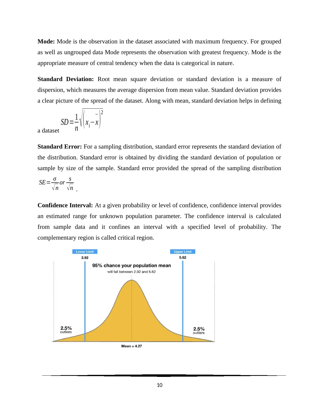
This document presents a comprehensive solution to a statistics homework assignment focusing on quantitative methods. It includes multiple-choice questions covering topics such as multivariate analysis, measures of central tendency (mean, median, mode), standard deviation, confidence intervals, and hypothesis testing. The solutions are detailed and provide explanations for each answer, referencing statistical rules and theorems where applicable. Key concepts like the Central Limit Theorem, p-values, and the Chi-Square test are also addressed. The assignment also includes definitions of statistical terms such as mean, median, mode, standard deviation, standard error and confidence interval. Desklib provides a platform for students to access this and other solved assignments and past papers.

Homework Statistics
1

1 C 26 C
2 C 27 C
3 D 28 C
4 D 29 D
5 12 30
6 D 31 A
7 D 32 B
8 33 C
9 C 34 A
10 E 35 D
11 A 36 B
12 C 37 B
13 C 38 C
14 D 39 B
15 C 40 A
16 A 41 D
17 D 42 B
18 A 43 A
19 B 44 C
20 B 45 D
21 D 46 A
22 D 47 B
23 A 48 D
24 D 49 D
25 C 50 A
MCQ OPTIONS
2

1. Multivariate Analysis is related to more than one outcome variables. Hence, relationship
between types of undergraduate major and positions held in business is the appropriate
example of multivariate analysis. (c)
2. Mode is the most frequent attribute in either grouped or ungrouped data. (c)
3. Standard deviation measures dispersion of a data set. Zero standard deviation is also
possible if the observations are identical or homogeneous in nature. Hence, (d) is the
correct answer.
4. For categorical data with two levels, mode is the best measure of central tendency. (d)
5. Arranging the data in ascending order, we get the sequence: 7, 8, 9, 11, 12, 13, 14, 15, 17,
where number of observations =9 (odd). Hence, median is the ( 9+1
2 ) th=5 th
observation
= 12
6. The mean number of faculties in a department will be
( 7+8+9+ 11+ 12+13+ 14+15+17
9 )=11 .78
, (d)
7. To test whether blondes have more fun than non-blondes, we need to compare column
wise and the required percentages would be calculated row wise (across) (d)
8. S
9. Measures of dispersion, such as standard deviation or mean deviation signify the spread
of the data from mean position. (c)
10. The percentage of males arrested for violent crime was 20%. But, there was not enough
information for finding percentage of males committing violent crime.
11. Concerning the data presented in question 10, cases were divided by sex, and the
percentages were done on the columns. Hence, row wise comparison was possible. It was
possible to say that males or females committed more properly crimes than violent
crimes. But, column wise comparison was not possible. (a)
12. Mean has restriction for outlier values, mode can not a meaning full attribute in
continuous data. But, median can be used for any level of measurement. (c)
13. The mean was ( 18+33+7+ 32+6+5+ 4
7 )=15
,(C)
3

14. Mean, median both are good measures of central tendency for continuous data. Standard
deviation can measure spread of the data for continuous type of data. (d)
15. The 68% confidence interval for the sample mean with sample standard error is
calculated as x
−
±tcrit∗SE=22±1. 6604∗5=[ 13. 698 , 30. 302 ] . Hence, most suitable choice
was option (C)
16. In Descriptive Statistics, we organize and represent data in suitable format. (a)
17. A population is a complete set of individuals. A Sample is a sub set of individuals. (d)
18. Parameter and statistic are related to population and sample. But, any characteristic of an
environment or object can be measured by a variable. (a)
19. From definition, Statistic measures characteristic of a sample. (b)
20. Total frequency = 1+3+5+3+5+5+1+ 2=25 from the histogram. Now, schools below
15% acceptance rate = 1. Hence, percentage =
1
25 =0 .04=4 % (b)
21. Number of schools over 30% acceptance = 5+5+1+2=13 from histogram. (d)
22. For skewed distribution median is the best choice as measure of central tendency. The
aim was to show that baseball players were overpaid, and for this purpose neither mean,
nor mode would be appropriate. (d)
23. Total frequency = 667, and the median would be at
667
2 =333 .5 th observation which
corresponds to the next higher value. In this case it was 334 corresponding to age 20. (a)
Age Students Cumulative Freq
18 14 14
19 120 134
20 200 334
21 200 534
22 90 624
23 30 654
24 10 664
25 2 666
32 1 667 N
4

24. Properties of normal curve are, 1) curve is symmetric, 2) peak is at the center, which is
the mean of the distribution, 3) the spread of the curve is in accordance with the standard
deviation (d)
25. Population mean = 68, SD = 9, Now, X =77 is at μ+σ level. Now using 68-95-99.7
rule, we get P ( X≤77 ) =2 .35 % +13. 5 %+68 %=83 .85 % . So, required probability
P ( X >77 ) =100 %−83. 85 %=16 . 15 % ,nearest answer (c)
5

26. Population mean = 70 min, SD = 10 min, Now, X =90 is at μ+2 σ level. Now using 68-
95-99.7 rule, we get P ( X≤90 ) =2 .35 %+13 .5 % +68 %+13 . 5=97 .35 % . So, required
percentage students who will not be able to finish = P ( X >90 ) =2. 65 % , (c)
27. P ( Z <1. 15 ) =0 .5+ P ( 0< Z <1. 15 ) =0. 5+0 . 3749=0 . 8749 (Using standard normal table) (C)
28. P ( −0 .5< Z <1. 2 ) =P ( Z<1 . 2 ) −P ( Z <−0 . 5 ) =0. 8849−0 .3085=0 .5764 (C)
29. Let X ~ N ( 15 ,32 ) where X denotes the time taken for the computer link. Now for 90%
occasions the computer link is made following the probability P ( X < x ) =0 . 9 .
So,
P ( X < x ) =0 . 9 => P ( Z < x−15
3 )=0. 9 => P ( Z <x−15
3 ) =P ( Z <1. 2815 )
=> x−15
3 =1. 2815 => x=18. 84 sec onds . ( d )
30. D
31. Let X ~ N ( 202, 32 ) be the weights of cookie packets. According to problem,
P ( X < x ) =0 . 01=> P ( Z< x−202
3 )=0 . 01=> P ( Z< x−202
3 ) =P ( Z <−2 .326 )
=> x=202−3∗2 . 326=> 208 . 98 (a )
32. Central limit theorem: This says that if the sample size is large ( n≥30 ) then the sampling
distribution of the mean follows normal distribution. (b)
33. Required probability
P ( x
¿
>6 .1 ) =P
( Z > 6 .1−6
2. 2
√ 400 ) =P ( Z >0 . 909 ) =1−P ( Z< 0 .909 ) =0 . 1816
(C)
34. Standard deviation of sampling distribution of x
¿
is
σ
√ n =770
10 =$ 77 . 0
and
mean=μ=$ 1520 ( A )
35. Required probability
P ( x
¿
<1500 ) =P
( Z< 1500−1520
77
√ 100 )=P ( z<−20
7 . 7 )=P ( Z <−2 . 597 ) =0 . 00469
(using standard
normal table) (d)
6

36. At 90% level, z=1 .645 and the confidence interval for estimating the unknown
population mean is
80±1. 645∗20
√ 100 =80±3. 29
(b)
37. Margin of error is calculated as
zcrit∗ σ
√ n , hence for increase in sample size (n) the
margin of error decreases. (b)
38. At 95% level, z=1 .96 and the confidence interval for estimating the unknown population
mean is
50±1 . 96∗ 5
√ 25 =50±1. 96=[ 48 . 04 , 51. 96 ] (c)
39. Margin of error decreases with increase in sample size at any given confidence level. (b)
40. At 99% level, z=2 .576 and the confidence interval for estimating the unknown
population mean is
65±2. 576∗ 2 . 4
√ 36 =65±1. 0304
(a)
41. Margin of error is calculated as
zcrit∗ σ
√ n =±1=> 2. 576∗2 . 4
√ n =±1=> n= ( ±2 .576∗2 . 4 ) 2=38 .22
,(d)
42. At 95% level, z=1 .96 and the confidence interval for estimating the unknown population
mean is
8±1. 96∗ 5
√ 100 =8±0 . 98
(b)
43. Test statistic
z= x
¿
−μ
σ
√ n
=17−20
6
√ 9
=−1 . 5
, and the p-value for
=P ( z<−1. 5 ) =P ( z >1 .5 ) =0 .0668 (using z table) (a)
44. For statistical significance, p-value should be smaller than the level of significance. (c)
45. P-value signifies the smallest level of probability or significance at which null hypothesis
can be rejected (Imbens, & Kolesar, 2016).(D)
7

46. We have to test one tail (left) hypothesis. Test statistic
z= x
−
−μ
σ / √ n = 9 .6−10
0 . 4/ 5 =−5
So, p-value is P ( Z <−5 ) =0 .00000 (a) (Ross, 2017)
47. Let X ~ N ( 70 ,152 ) be the time required. Sample size n=9 . Test statistic
z= x
−
−μ
σ / √ n =64−70
15/3 =−1 .2 and the p-value P ( Z <−1 .2 ) =0 .115 > α=0 . 01
Hence, H0 should not be rejected at 1% level of significance. For rejection of H0 we need
p-value to be less than α ( D’Agostino, 2017)(B)
48. At 90% level, z=1 .645 and the confidence interval for estimating the unknown
population mean is
64±1. 645∗15
√ 9 =64±8. 225
, so nearest answer (d)
8

49. Standard error
SE= σ
√ n =27 .839
√ 3 =16 . 07(d )
where
x
¿
=260+315+295
3 =290
σ = √ ( 260−290 ) 2+ ( 315−290 ) 2+ ( 295−290 ) 2
3 =27 .839 (Chatfield, 2018).
50. P-value =P (|t|>1 .93 ) =0 . 0695 at 18 degrees of freedom. Hence, p-value < α =0 . 10 and
we reject null hypothesis at α =0 . 10 . (a)
Standard Definitions
Mean: Mean can be measured as the arithmetic mean, geometric mean, and harmonic mean.
The arithmetic mean is calculated by taking average or dividing the sum of all observations by
number of observations
( x
¿
=
∑
i
xi
N ) . One of the drawbacks is that the arithmetic mean gets easily
affected by outlier or abrupt large observation values.
The geometric mean is calculated as the nth (no of observations) root of the product of the
observations GM =n
√ x1 . x2 . x3 .. . xn .
The harmonic mean is calculated as the arithmetic mean of the inverse of the observations
( HM = n
1
x1
+ 1
x2
+.. . .+ 1
xn ) .
Median: Median is the middlemost observation of any dataset or number of observations.
Median splits the dataset in two parts, below 50% and above 50% observations. Median is
considered as the geometrical average of a dataset. Median is a better measure of central
tendency compared to mean for open end data and dataset with considerable outliers.
9

Mode: Mode is the observation in the dataset associated with maximum frequency. For grouped
as well as ungrouped data Mode represents the observation with greatest frequency. Mode is the
appropriate measure of central tendency when the data is categorical in nature.
Standard Deviation: Root mean square deviation or standard deviation is a measure of
dispersion, which measures the average dispersion from mean value. Standard deviation provides
a clear picture of the spread of the dataset. Along with mean, standard deviation helps in defining
a dataset
SD= 1
n √ ( xi−x
−
) 2
Standard Error: For a sampling distribution, standard error represents the standard deviation of
the distribution. Standard error is obtained by dividing the standard deviation of population or
sample by size of the sample. Standard error provided the spread of the sampling distribution
SE= σ
√ n or s
√ n .
Confidence Interval: At a given probability or level of confidence, confidence interval provides
an estimated range for unknown population parameter. The confidence interval is calculated
from sample data and it confines an interval with a specified level of probability. The
complementary region is called critical region.
10

References
Chatfield, C. (2018). Statistics for technology: a course in applied statistics. Routledge.
D’Agostino, R. B. (2017). Tests for the normal distribution. In Goodness-of-fit-techniques (pp.
367-420). Routledge.
Imbens, G. W., & Kolesar, M. (2016). Robust standard errors in small samples: Some practical
advice. Review of Economics and Statistics, 98(4), 701-712.
Ross, A. (2017). Area Under the Normal Curve. In Pedagogy and Content in Middle and High
School Mathematics (pp. 131-140). SensePublishers, Rotterdam.
11