Quantitative Reasoning and Analysis: Regression and Hypothesis Testing
VerifiedAdded on 2022/08/23
|19
|1667
|17
Homework Assignment
AI Summary
This assignment delves into quantitative reasoning and statistical analysis, covering key concepts such as time series analysis, simple linear regression, and hypothesis testing. The assignment begins with an examination of time series, using craft beer production data to calculate and interpret index numbers, and comparing different base periods. It then moves on to simple linear regression, analyzing relationships between variables like median salary and academic reputation, and unemployment rate with GDP and inflation. The assignment also explores hypothesis testing, with examples involving proportions and means, and includes detailed calculations, interpretations, and conclusions. Data from various sources, including worldbank.org and statcan.gc.ca, are used to support the analyses. The document provides comprehensive solutions to each section, demonstrating statistical techniques and their applications.

Running head: QUANTITIVE REASONING AND ANALYSIS
Quantitive Reasoning and Analysis
Name of the Student
Name of the University
Course ID
Quantitive Reasoning and Analysis
Name of the Student
Name of the University
Course ID
Paraphrase This Document
Need a fresh take? Get an instant paraphrase of this document with our AI Paraphraser
1QUANTITIVE REASONING AND ANALYSIS
Table of Contents
Section one: Time Series.................................................................................................................2
Question 1.1.................................................................................................................................2
Question 1.2.................................................................................................................................2
Question 1.3.................................................................................................................................3
Question 1.4.................................................................................................................................4
Question 1.5.................................................................................................................................5
Section two: Simple Linear Regression...........................................................................................6
Question 2.1.................................................................................................................................6
Question 2.2.................................................................................................................................7
Question 2.3.................................................................................................................................7
Question 2.4.....................................................................................................................................9
Question 2.5.....................................................................................................................................9
Section 3: Hypothesis and test.......................................................................................................10
Question 3.1...............................................................................................................................10
Question 3.2...............................................................................................................................13
References......................................................................................................................................16
2QUANTITIVE REASONING AND ANALYSIS
Section one: Time Series
Question 1.1
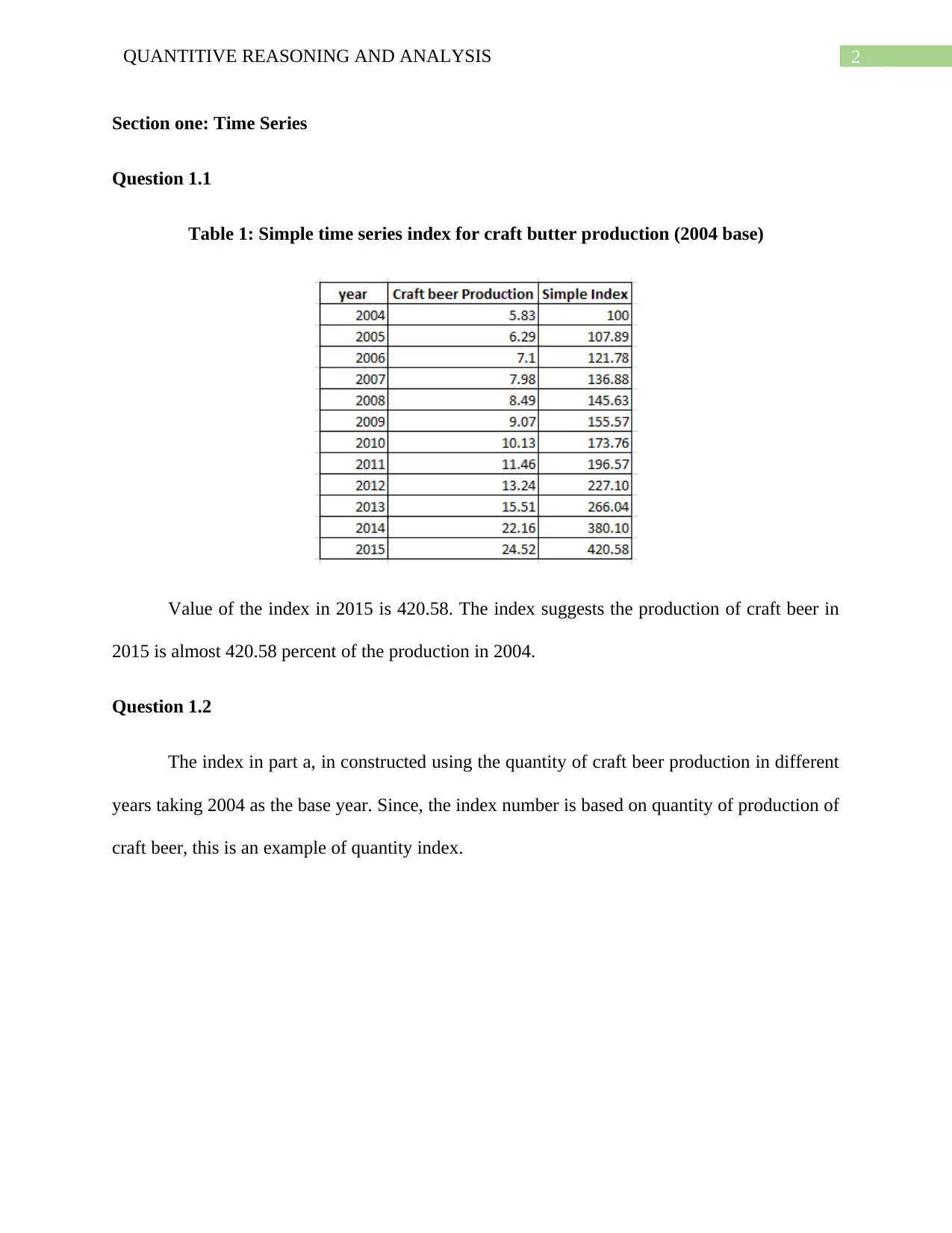
Table 1: Simple time series index for craft butter production (2004 base)
Value of the index in 2015 is 420.58. The index suggests the production of craft beer in
2015 is almost 420.58 percent of the production in 2004.
Question 1.2
The index in part a, in constructed using the quantity of craft beer production in different
years taking 2004 as the base year. Since, the index number is based on quantity of production of
craft beer, this is an example of quantity index.
⊘ This is a preview!⊘
Do you want full access?
Subscribe today to unlock all pages.

Trusted by 1+ million students worldwide
3QUANTITIVE REASONING AND ANALYSIS
Question 1.3
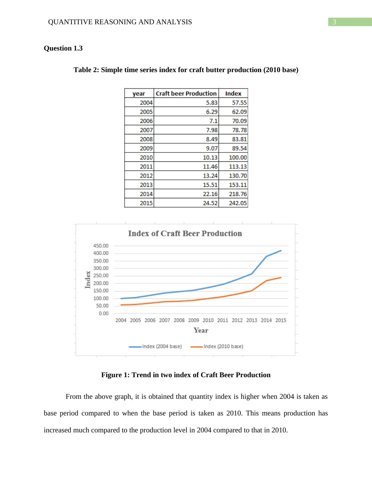
Table 2: Simple time series index for craft butter production (2010 base)
Figure 1: Trend in two index of Craft Beer Production
From the above graph, it is obtained that quantity index is higher when 2004 is taken as
base period compared to when the base period is taken as 2010. This means production has
increased much compared to the production level in 2004 compared to that in 2010.
Paraphrase This Document
Need a fresh take? Get an instant paraphrase of this document with our AI Paraphraser
4QUANTITIVE REASONING AND ANALYSIS
Question 1.4
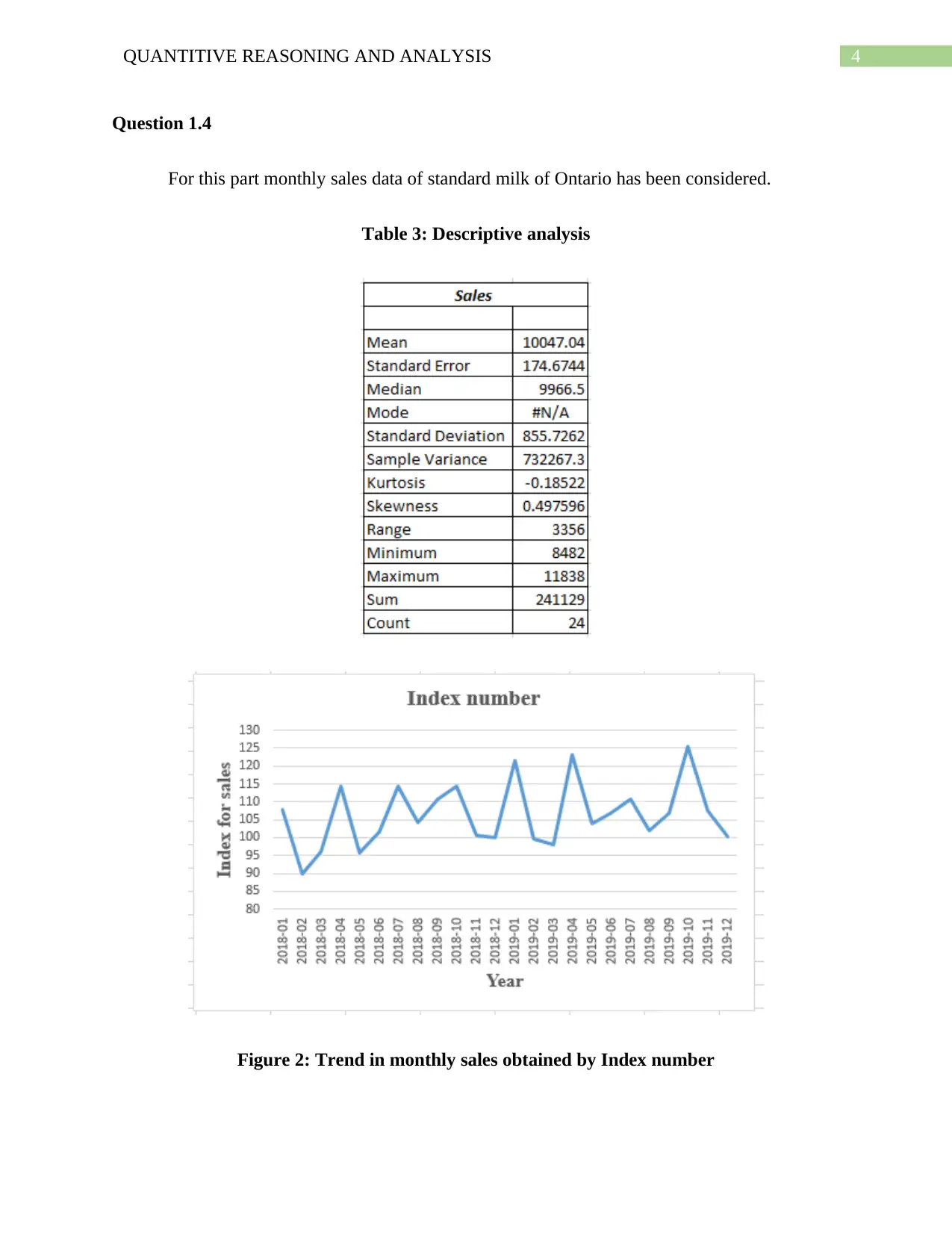
For this part monthly sales data of standard milk of Ontario has been considered.
Table 3: Descriptive analysis
Figure 2: Trend in monthly sales obtained by Index number
Question 1.4
For this part monthly sales data of standard milk of Ontario has been considered.
Table 3: Descriptive analysis
Figure 2: Trend in monthly sales obtained by Index number
5QUANTITIVE REASONING AND ANALYSIS
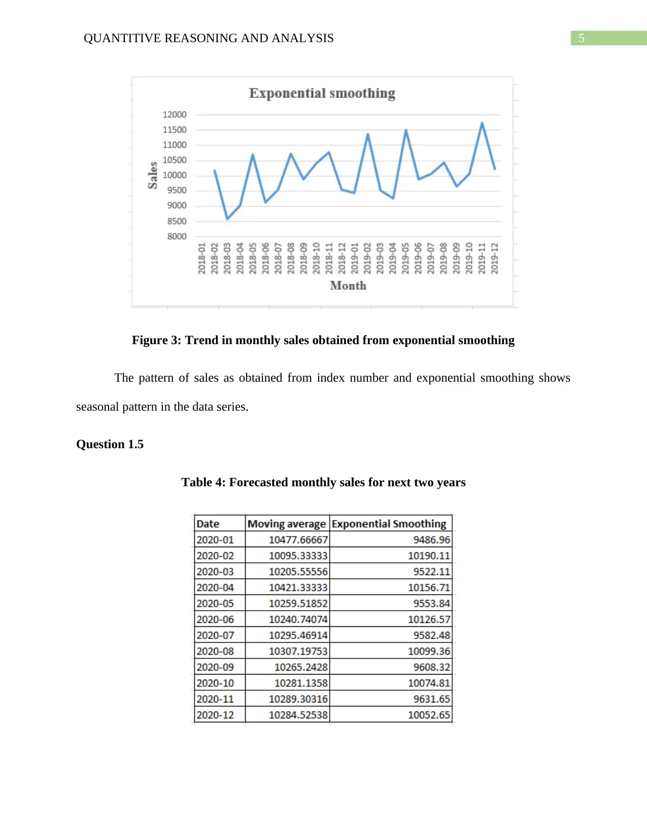
Figure 3: Trend in monthly sales obtained from exponential smoothing
The pattern of sales as obtained from index number and exponential smoothing shows
seasonal pattern in the data series.
Question 1.5
Table 4: Forecasted monthly sales for next two years
Figure 3: Trend in monthly sales obtained from exponential smoothing
The pattern of sales as obtained from index number and exponential smoothing shows
seasonal pattern in the data series.
Question 1.5
Table 4: Forecasted monthly sales for next two years
⊘ This is a preview!⊘
Do you want full access?
Subscribe today to unlock all pages.

Trusted by 1+ million students worldwide
6QUANTITIVE REASONING AND ANALYSIS
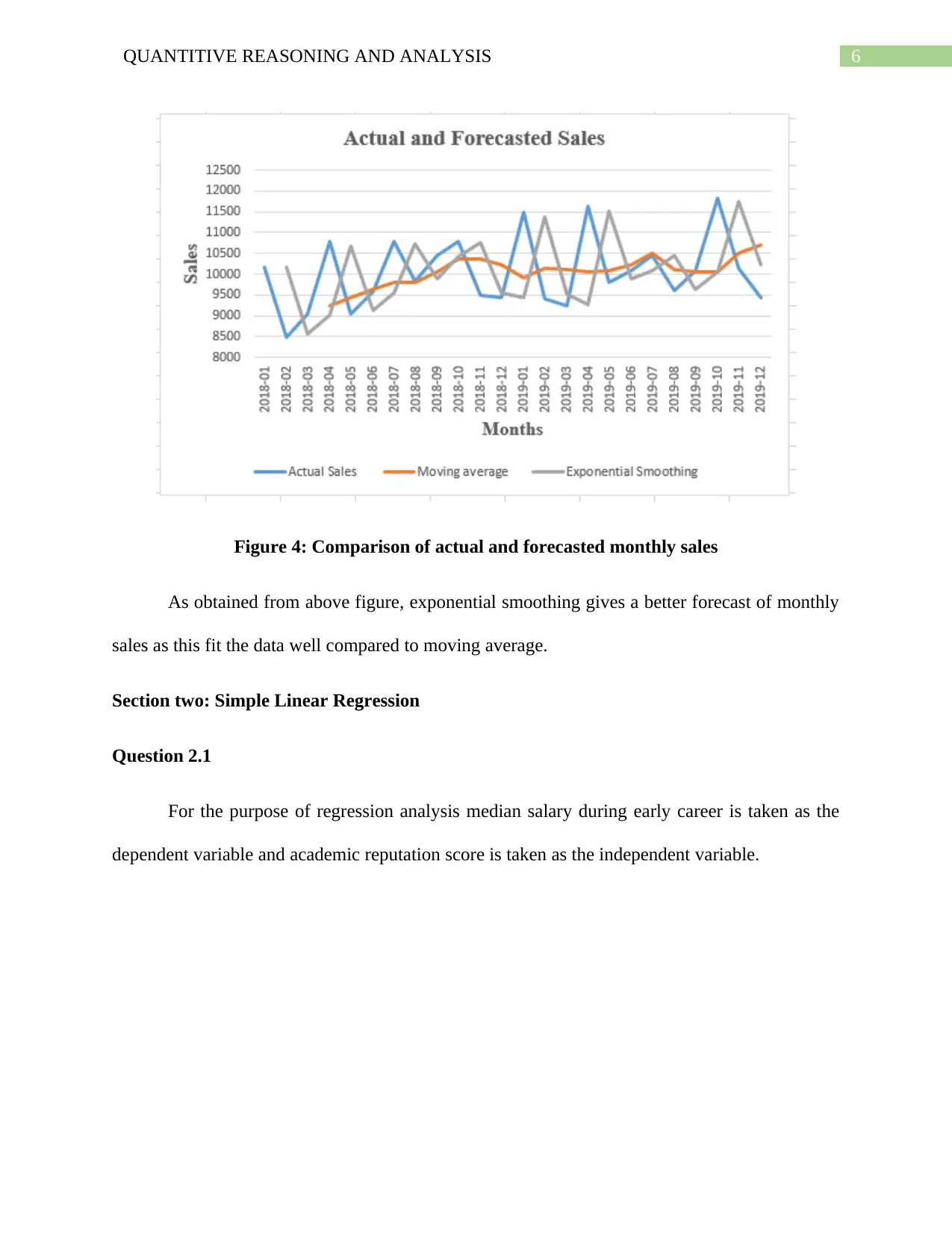
Figure 4: Comparison of actual and forecasted monthly sales
As obtained from above figure, exponential smoothing gives a better forecast of monthly
sales as this fit the data well compared to moving average.
Section two: Simple Linear Regression
Question 2.1
For the purpose of regression analysis median salary during early career is taken as the
dependent variable and academic reputation score is taken as the independent variable.
Paraphrase This Document
Need a fresh take? Get an instant paraphrase of this document with our AI Paraphraser
7QUANTITIVE REASONING AND ANALYSIS
Question 2.2
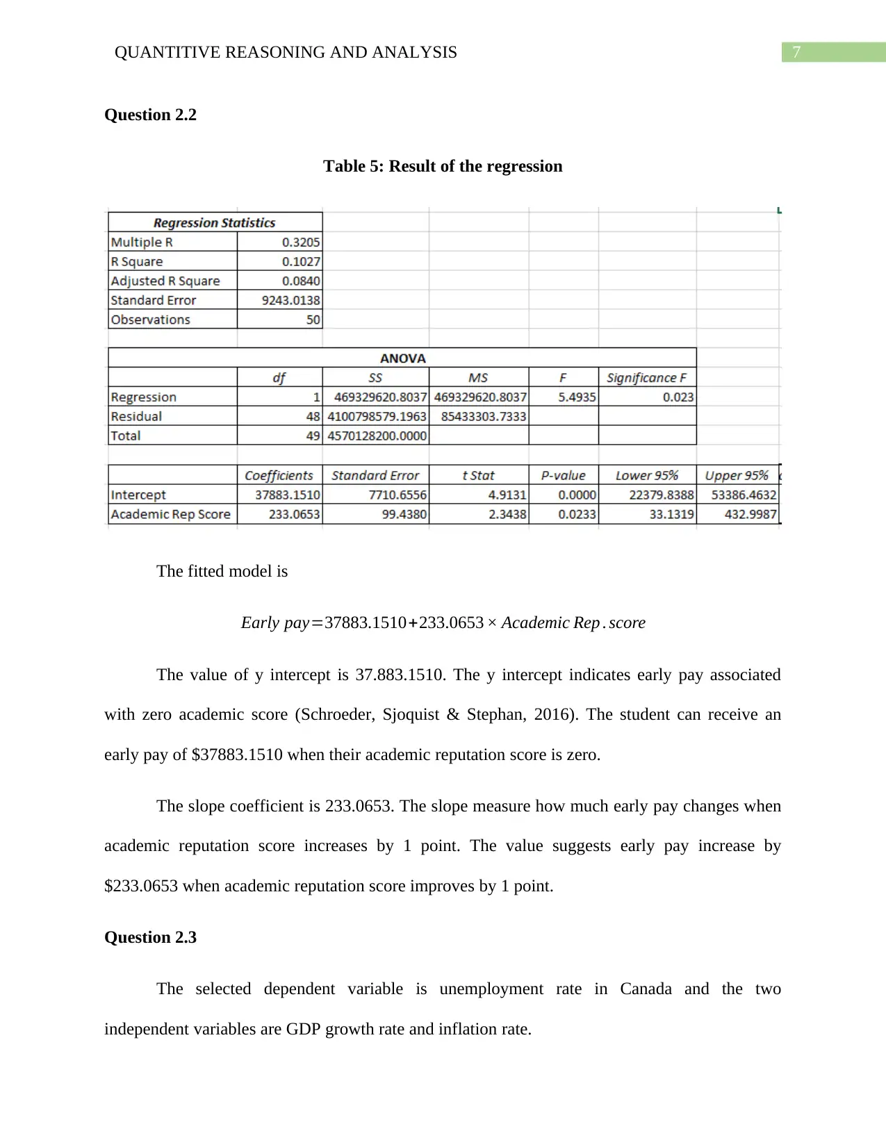
Table 5: Result of the regression
The fitted model is
Early pay=37883.1510+233.0653 × Academic Rep . score
The value of y intercept is 37.883.1510. The y intercept indicates early pay associated
with zero academic score (Schroeder, Sjoquist & Stephan, 2016). The student can receive an
early pay of $37883.1510 when their academic reputation score is zero.
The slope coefficient is 233.0653. The slope measure how much early pay changes when
academic reputation score increases by 1 point. The value suggests early pay increase by
$233.0653 when academic reputation score improves by 1 point.
Question 2.3
The selected dependent variable is unemployment rate in Canada and the two
independent variables are GDP growth rate and inflation rate.
8QUANTITIVE REASONING AND ANALYSIS
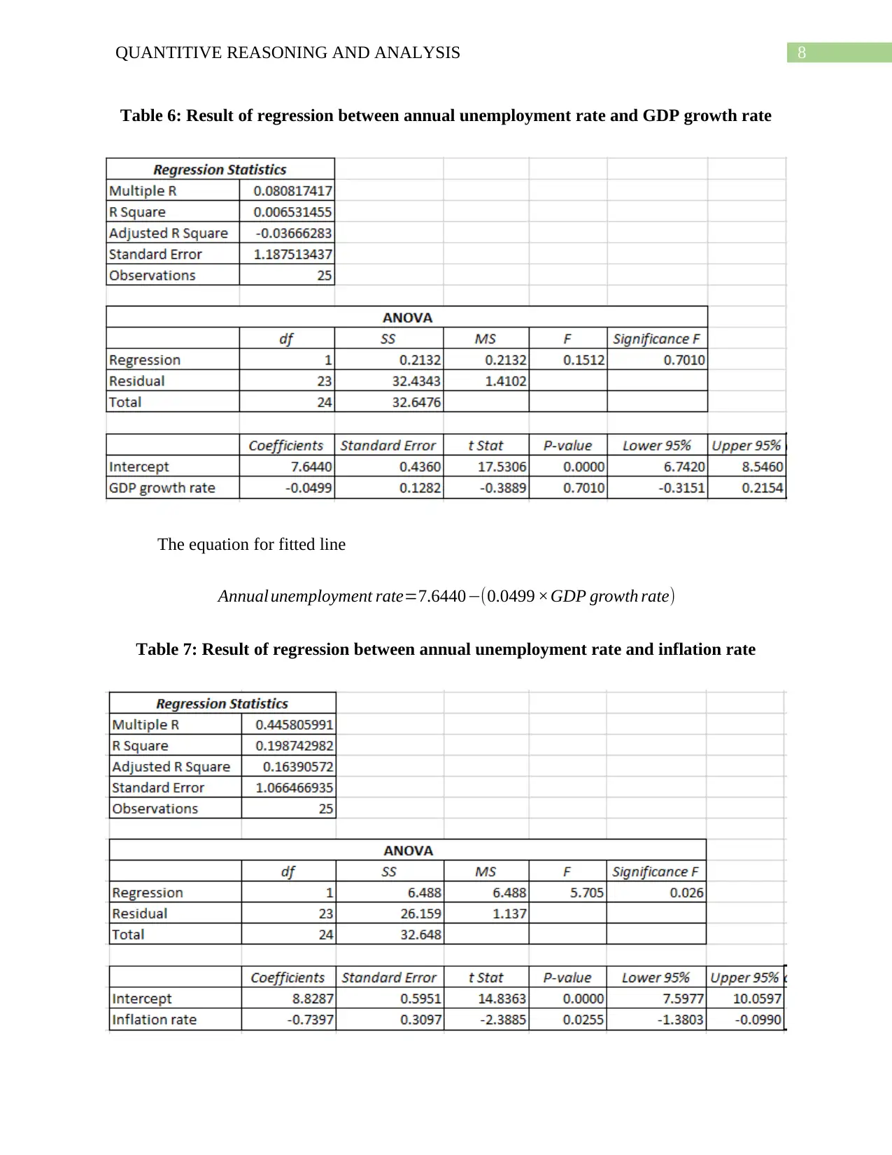
Table 6: Result of regression between annual unemployment rate and GDP growth rate
The equation for fitted line
Annual unemployment rate=7.6440−(0.0499 ×GDP growth rate)
Table 7: Result of regression between annual unemployment rate and inflation rate
Table 6: Result of regression between annual unemployment rate and GDP growth rate
The equation for fitted line
Annual unemployment rate=7.6440−(0.0499 ×GDP growth rate)
Table 7: Result of regression between annual unemployment rate and inflation rate
⊘ This is a preview!⊘
Do you want full access?
Subscribe today to unlock all pages.

Trusted by 1+ million students worldwide
9QUANTITIVE REASONING AND ANALYSIS
The equation for fitted line
Annual unemployment rate=8.8287−(0.7397 ×GDP growthrate)
Question 2.4
For the first model the slope for GDP growth is -0.0499. The slope coefficient suggests
that unemployment decreases by 0.05 percent given 1 percent increase in GDP growth rate
(Darlington & Hayes, 2016) p value for the coefficient is 0.7010 which is greater than the
significance value. This suggests acceptance of the null hypothesis that 𝛽1 = 0.
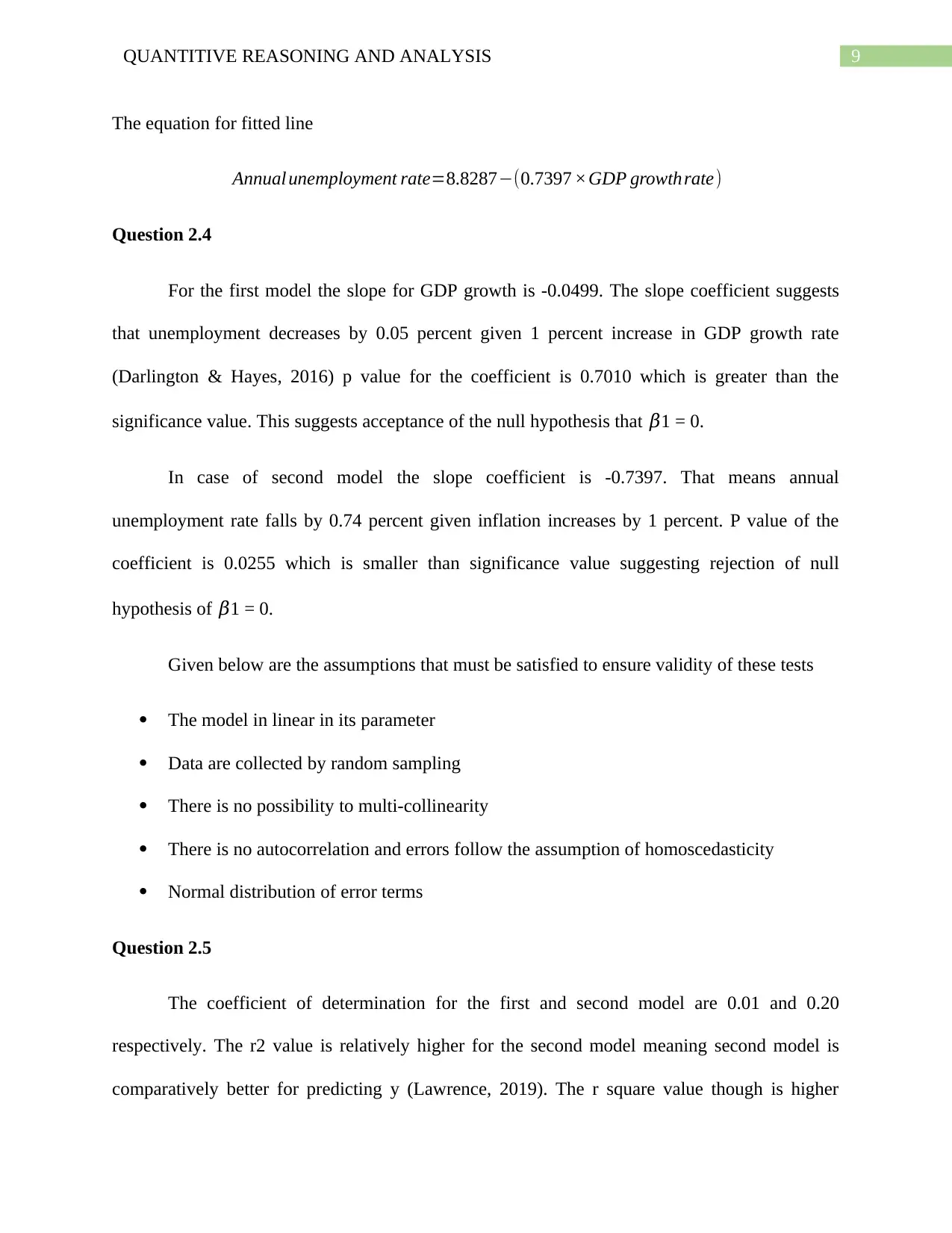
In case of second model the slope coefficient is -0.7397. That means annual
unemployment rate falls by 0.74 percent given inflation increases by 1 percent. P value of the
coefficient is 0.0255 which is smaller than significance value suggesting rejection of null
hypothesis of 𝛽1 = 0.
Given below are the assumptions that must be satisfied to ensure validity of these tests
The model in linear in its parameter
Data are collected by random sampling
There is no possibility to multi-collinearity
There is no autocorrelation and errors follow the assumption of homoscedasticity
Normal distribution of error terms
Question 2.5
The coefficient of determination for the first and second model are 0.01 and 0.20
respectively. The r2 value is relatively higher for the second model meaning second model is
comparatively better for predicting y (Lawrence, 2019). The r square value though is higher
Paraphrase This Document
Need a fresh take? Get an instant paraphrase of this document with our AI Paraphraser
10QUANTITIVE REASONING AND ANALYSIS
compared to the first model however overall the r2 value is very low meaning fitness is not good.
The explanatory variable (inflation) in the second model is statistically significant indicating
inflation is a significant predictor of unemployment rate. Other factors however need to be
included to get a better prediction of unemployment rate.
Section 3: Hypothesis and test
Question 3.1
a)
Sample proportion of Mexican American among U.S. Hispanics is (575/850) = 0.6765
Hypotheses
Null hypothesis: Proportion of Mexican American among U.S. Hispanics is 0.63
H0 : P=0.63
Alternative hypothesis: Proportion of Mexican American among U.S. Hispanics is not equal to
0.63
H1 : P ≠ 0.63
Level of significance
Chosen value of alpha is 0.05.
Test statistics
11QUANTITIVE REASONING AND ANALYSIS
Z= ^P−P
√ P (1−P )
n
¿ 0.6765−0.63
√ 0.63 ×0.37
850
¿ 0.0465
√0.000274
¿ 0.0465
0.0166
¿ 2.806
Conclusion
Critical z value corresponding to an alpha value of 0.05 is 1.96. The computed Z value is
greater than critical z implying rejection of null hypothesis (Bartee, 2019). From the test result, it
can therefore be conclude that the proportion of Mexican American among U.S. Hispanics is
different from 63%.
b)
Sample proportion of women in the Hispanic grocery shoppers is = 606/689 = 8795
Hypotheses
Null hypothesis: Proportion of women in Hispanics grocery shoppers is 0.94
H0 : P=0.94
⊘ This is a preview!⊘
Do you want full access?
Subscribe today to unlock all pages.

Trusted by 1+ million students worldwide
1 out of 19
Your All-in-One AI-Powered Toolkit for Academic Success.
+13062052269
info@desklib.com
Available 24*7 on WhatsApp / Email
![[object Object]](/_next/static/media/star-bottom.7253800d.svg)
Unlock your academic potential
Copyright © 2020–2026 A2Z Services. All Rights Reserved. Developed and managed by ZUCOL.
