RSM701 Quantitative Research I: Understanding Statistical Concepts

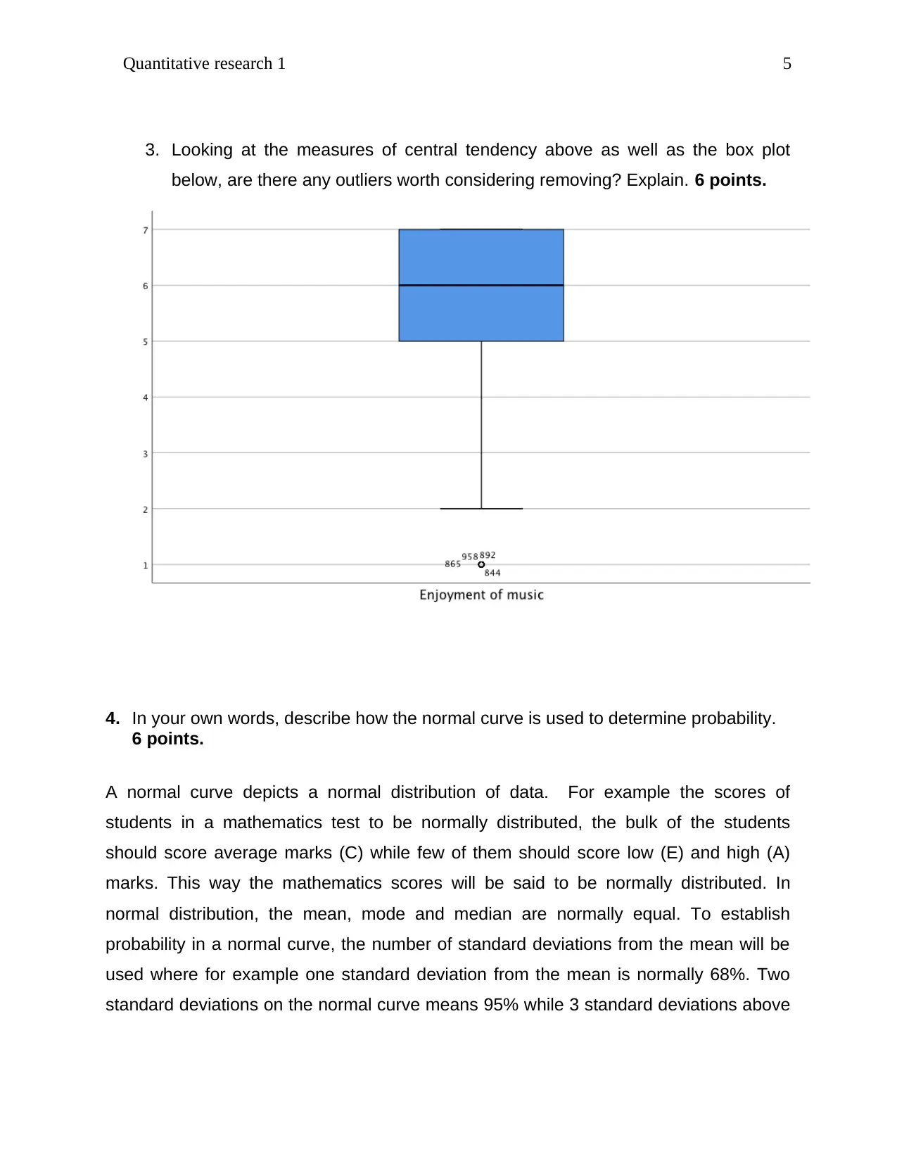
This assignment solution for RSM701 Quantitative Research I covers various statistical concepts, including identifying samples and types of statistics (descriptive vs. inferential) in different scenarios, determining independent and dependent variables, and understanding measurement types. It analyzes measures of central tendency, skewness, and data distribution using provided data, box plots, and histograms. The solution discusses the appropriateness of using the median versus the mean, explains variability in data sets, interprets p-values in hypothesis testing, and justifies the use of samples to generalize to a population. The document also references relevant research articles to support its explanations. Desklib provides this and other solved assignments for students.

Quantitative research 1 1
RSM701
Quantitative Research I
Student name:
Tutor name:

Quantitative research 1 2
a. George is interested in how four kinds of nutrition supplements
effect body builders’ weight loss.
Sample: body builders
Statistics: Inferential
How you know: George is not interested in the descriptive statistics such as measures
of central tendency but interested in the relationship that exists between nutrition types
and weight of body builders.
Independent Variable and Measurement Type: Nutrition type, nominal
Dependent Variable and Measurement Type: Weight, ratio
b. Jason measures math knowledge of his fellow statistics students.
Sample: Statistics students
Statistics: Descriptive statistics
How you know: This is because there is only one variable that Jason wants to
measure. He is not doing any correlation or relationship since there is only one variable.
Independent Variable and Measurement Type: N/A
Dependent Variable and Measurement Type:
c. Tia wants to know how 4th and 5th grades respond differently to
negative feedback.
Sample: 4th and 5th grade students
Statistics: Inferential
How you know: Tia is interested in the relationship that exists between the two grades
and negative feedback. (The relationship between grades and negative feedback)
Independent Variable and Measurement Type: Negative feedback
Dependent Variable and Measurement Type: Response

Quantitative research 1 3
2. Adults’ enjoyment of music was measured on a 7-point scale, with a 7
representing the highest level of music enjoyment. Measures of central
tendency, a box plot, and a histogram are included below.
Enjoyment of music
N Valid 1000
Missing 0
Mean 5.50
Median 6.00
Mode 7
Std. Deviation 1.536
Variance 2.360
Skewness -.975
Std. Error of Skewness .077
Kurtosis .329
Std. Error of Kurtosis .155
Table 1

Quantitative research 1 4
Figure 1
From table 1 above, it can be observed that the mean enjoyment level was 5.5, median
enjoyment level was 6 while the mode enjoyment level was 7. This indicates that music
enjoyment among the adults was above average (3.5). A standard deviation of 1.54
showed that the variation of music enjoyment was 1.54 units above or below the mean
(5.5± 1.54 ¿ . The distribution curve is observed to be skewed to the right. This means
that the enjoyment levels among the adults is not normally distributed. This is because
more adults showed highest level of music enjoyment while few adults showed low
levels of music enjoyment. Measures of central tendency will be similar where the data
is normally distributed and not similar where the data is not normally distributed (Leigh,
2008).

Quantitative research 1 5
3. Looking at the measures of central tendency above as well as the box plot
below, are there any outliers worth considering removing? Explain. 6 points.
4. In your own words, describe how the normal curve is used to determine probability.
6 points.
A normal curve depicts a normal distribution of data. For example the scores of
students in a mathematics test to be normally distributed, the bulk of the students
should score average marks (C) while few of them should score low (E) and high (A)
marks. This way the mathematics scores will be said to be normally distributed. In
normal distribution, the mean, mode and median are normally equal. To establish
probability in a normal curve, the number of standard deviations from the mean will be
used where for example one standard deviation from the mean is normally 68%. Two
standard deviations on the normal curve means 95% while 3 standard deviations above

Quantitative research 1 6
the mean means 99.7%. However, other standard deviations which are also known as
Z-scores can be interpreted from the normal tables to get the probabilities.
5 Give an example of data for each of the following and explain why:
a. When the median is more appropriate to use than the mean (3 points)
The median is more appropriate where the data has outliers hence not normally
distributed.
Example: 2, 4, 5, 7, 8, 10, 11, 13, 14, 16, 17, 434
b. When the mean is more appropriate to use than the median (3 points)
The mean is more appropriate where the data is large and has no outliers hence
normally distributed (Derrick, Toher, & White, 2017).
Example: 2, 4, 5, 7, 8, 10, 11, 13, 14, 16, 17, 19, 21, 22, 23, 25, 26, 28, 30, 33, 35, 35
6 Give an example of data for each of the following and explain why:
a. When you would expect high variability (3 points)
High variability is expected in a data set that has values that are highly spread apart.
Since variability is a measure of central tendency, when the data points are far apart,
the deviation from the mean also tend to be high hence high variability (Gelman, 2005).
Example of the data set is as below in a range of 1 to 200;
1, 35, 70, 120, 170, 200
b. When you would expect low variability (3 points)
Low variability is expected in a data set that has values that are close to each other.
Since variability is a measure of central tendency, when the data points are closer to
each other, the deviation from the mean tend to be lower hence low variability
(Hinkelmann & Kempthorne, 2010). Example of the data set is as below in a range of 1
to 20;

Quantitative research 1 7
2, 4, 6, 8, 10, 12, 14, 16, 18, 20
7 If p < 0.01, what does this mean? (6 points)
When the p-value is less than 0.01, it means that a given set of data is not consistent
with the (assumption) status quo that the null hypothesis is true. In this case the null
hypothesis is rejected and the alternative hypothesis not rejected. Therefore the
alternative is taken to be true (Howell, 2007).
8 In hypothesis testing, explain why you are using a sample to generalize to a
population. (6 points)
It is always expensive and time consuming to conduct a research of the entire
population thus a random sample that resembles the population in terms of
characteristics is used a representative of the whole population. This sample is
assumed to accurately represent the other elements of the entire population.

Quantitative research 1 8
Reference
erric To er ite P o to compare t e mean o t o ample t at incl de pairedD k, B., h , D., & Wh , . (2017). H w h f w s s h u
o er ation and independent o er ationbs v s bs v s.
antitati e met od or P c olo
Qu v h s f sy h gy, 13(2), 120 -
126.
elman A Anal i o ariance it i more important t an e erG , . (2005). ys s f v ? Why s h v .
T e anal o tati tic
h s f S s s, 33, 1
- 53.
in elmann empt orneH k , K., & K h , O. (2010).
e i n and anal i o e periment
D s g
ys s f x s ed ol(5 ., V . 8).
o ellH w , D. C. (2007).
tati tical met od or P c olo
S s h s f sy h gy ed ol(3 ., V . 5).
ei on mer riteL gh, E. S. (2008). C su s.
ellin o American olida
S g f
H ys, 6(3), 106 - 191.