Applied Data Analysis: Repeated Measures ANOVA and SPSS Interpretation
VerifiedAdded on 2021/05/30
|12
|1982
|320
Homework Assignment
AI Summary
This assignment delves into the application of repeated measures ANOVA using SPSS for quantitative research. It begins with descriptive statistics, followed by an examination of Box’s test for equality of covariance matrices, and multivariate tests. The analysis proceeds to Mauchly's test of sphericity, tests of within-subjects effects, and Levene’s test for homogeneity of variance. Tests of between-subjects effects and multivariate tests are also conducted. The assignment demonstrates how to interpret the results of these tests, including the significance of changes in creativity scores over time and across different treatment groups. Furthermore, the inclusion of post hoc tests (Bonferroni) provides a detailed understanding of the specific treatment effects. The assignment also explores the use of profile plots to visualize the trends. A divertimento task discusses the differences between ANOVA and ANCOVA, and provides examples of how ANCOVA can be applied, as well as potential limitations.

1
Research Methods II
Quantitative Research Methods
Applied Data Analysis (with SPSS)
Task 10: Repeated Measure of ANOVA
Research Methods II
Quantitative Research Methods
Applied Data Analysis (with SPSS)
Task 10: Repeated Measure of ANOVA
Paraphrase This Document
Need a fresh take? Get an instant paraphrase of this document with our AI Paraphraser
2
Table of Contents
Task 2..........................................................................................................................................................3
Part I: Descriptive Statistic.......................................................................................................................3
Part II: Box’s Test.....................................................................................................................................4
Part III: Multivariate Test.........................................................................................................................4
Part IV: Mauchly's Test of Sphericity.......................................................................................................5
Part V: Tests of Within-Subjects Effects...................................................................................................5
Part VI: Levene’s Test..............................................................................................................................6
Part VIl: Test of Between Subjects Effects...............................................................................................6
Part VIII: Multivariate Tests.....................................................................................................................6
Post Hoc Test of Treatments:..................................................................................................................7
Conclusion...................................................................................................................................................8
Divertimento Task.......................................................................................................................................8
Appendix...................................................................................................................................................10
3
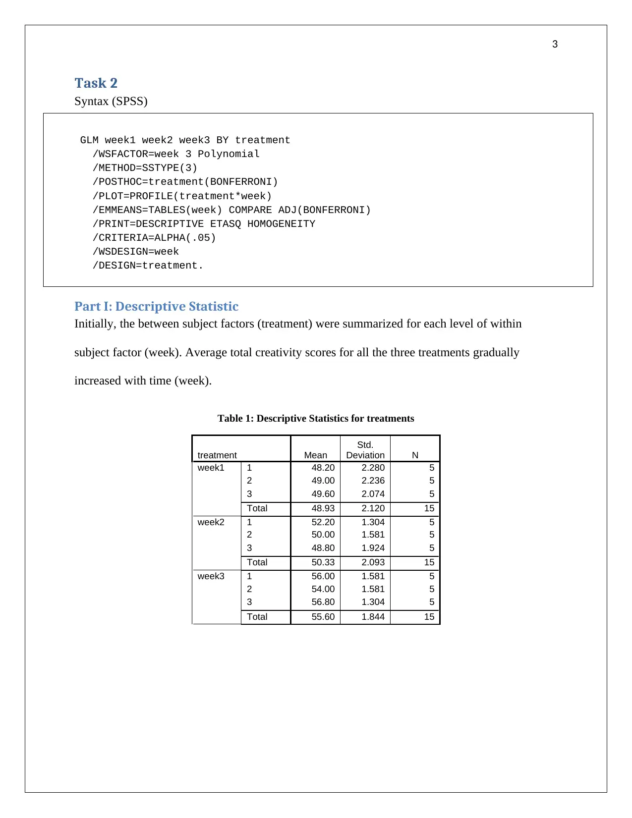
Task 2
Syntax (SPSS)
GLM week1 week2 week3 BY treatment
/WSFACTOR=week 3 Polynomial
/METHOD=SSTYPE(3)
/POSTHOC=treatment(BONFERRONI)
/PLOT=PROFILE(treatment*week)
/EMMEANS=TABLES(week) COMPARE ADJ(BONFERRONI)
/PRINT=DESCRIPTIVE ETASQ HOMOGENEITY
/CRITERIA=ALPHA(.05)
/WSDESIGN=week
/DESIGN=treatment.
Part I: Descriptive Statistic
Initially, the between subject factors (treatment) were summarized for each level of within
subject factor (week). Average total creativity scores for all the three treatments gradually
increased with time (week).
Table 1: Descriptive Statistics for treatments
treatment Mean
Std.
Deviation N
week1 1 48.20 2.280 5
2 49.00 2.236 5
3 49.60 2.074 5
Total 48.93 2.120 15
week2 1 52.20 1.304 5
2 50.00 1.581 5
3 48.80 1.924 5
Total 50.33 2.093 15
week3 1 56.00 1.581 5
2 54.00 1.581 5
3 56.80 1.304 5
Total 55.60 1.844 15
⊘ This is a preview!⊘
Do you want full access?
Subscribe today to unlock all pages.
Trusted by 1+ million students worldwide
4
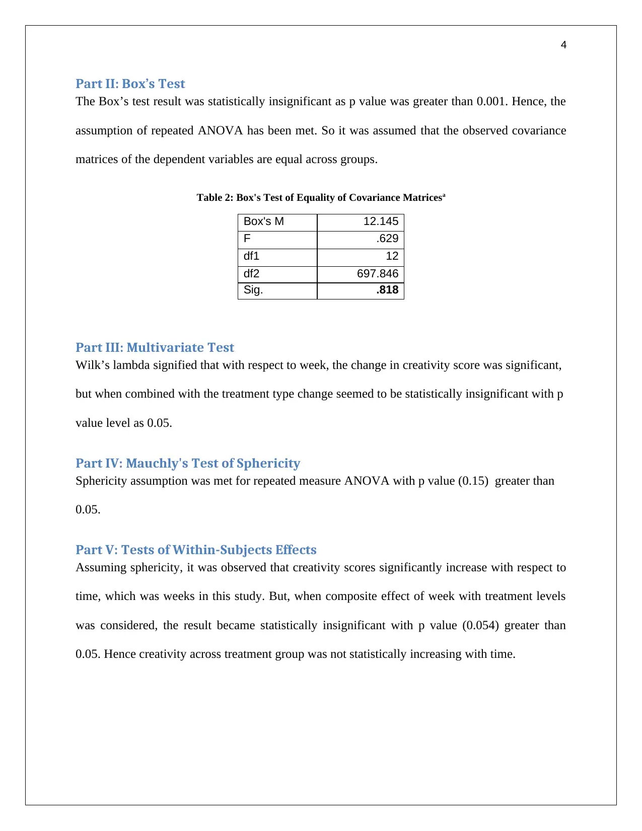
Part II: Box’s Test
The Box’s test result was statistically insignificant as p value was greater than 0.001. Hence, the
assumption of repeated ANOVA has been met. So it was assumed that the observed covariance
matrices of the dependent variables are equal across groups.
Table 2: Box's Test of Equality of Covariance Matricesa
Box's M 12.145
F .629
df1 12
df2 697.846
Sig. .818
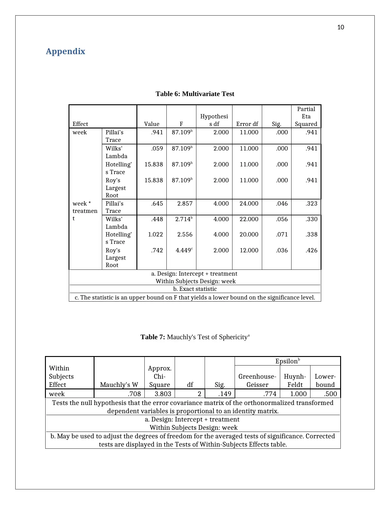
Part III: Multivariate Test
Wilk’s lambda signified that with respect to week, the change in creativity score was significant,
but when combined with the treatment type change seemed to be statistically insignificant with p
value level as 0.05.
Part IV: Mauchly's Test of Sphericity
Sphericity assumption was met for repeated measure ANOVA with p value (0.15) greater than
0.05.
Part V: Tests of Within-Subjects Effects
Assuming sphericity, it was observed that creativity scores significantly increase with respect to
time, which was weeks in this study. But, when composite effect of week with treatment levels
was considered, the result became statistically insignificant with p value (0.054) greater than
0.05. Hence creativity across treatment group was not statistically increasing with time.
Part II: Box’s Test
The Box’s test result was statistically insignificant as p value was greater than 0.001. Hence, the
assumption of repeated ANOVA has been met. So it was assumed that the observed covariance
matrices of the dependent variables are equal across groups.
Table 2: Box's Test of Equality of Covariance Matricesa
Box's M 12.145
F .629
df1 12
df2 697.846
Sig. .818
Part III: Multivariate Test
Wilk’s lambda signified that with respect to week, the change in creativity score was significant,
but when combined with the treatment type change seemed to be statistically insignificant with p
value level as 0.05.
Part IV: Mauchly's Test of Sphericity
Sphericity assumption was met for repeated measure ANOVA with p value (0.15) greater than
0.05.
Part V: Tests of Within-Subjects Effects
Assuming sphericity, it was observed that creativity scores significantly increase with respect to
time, which was weeks in this study. But, when composite effect of week with treatment levels
was considered, the result became statistically insignificant with p value (0.054) greater than
0.05. Hence creativity across treatment group was not statistically increasing with time.
Paraphrase This Document
Need a fresh take? Get an instant paraphrase of this document with our AI Paraphraser
5
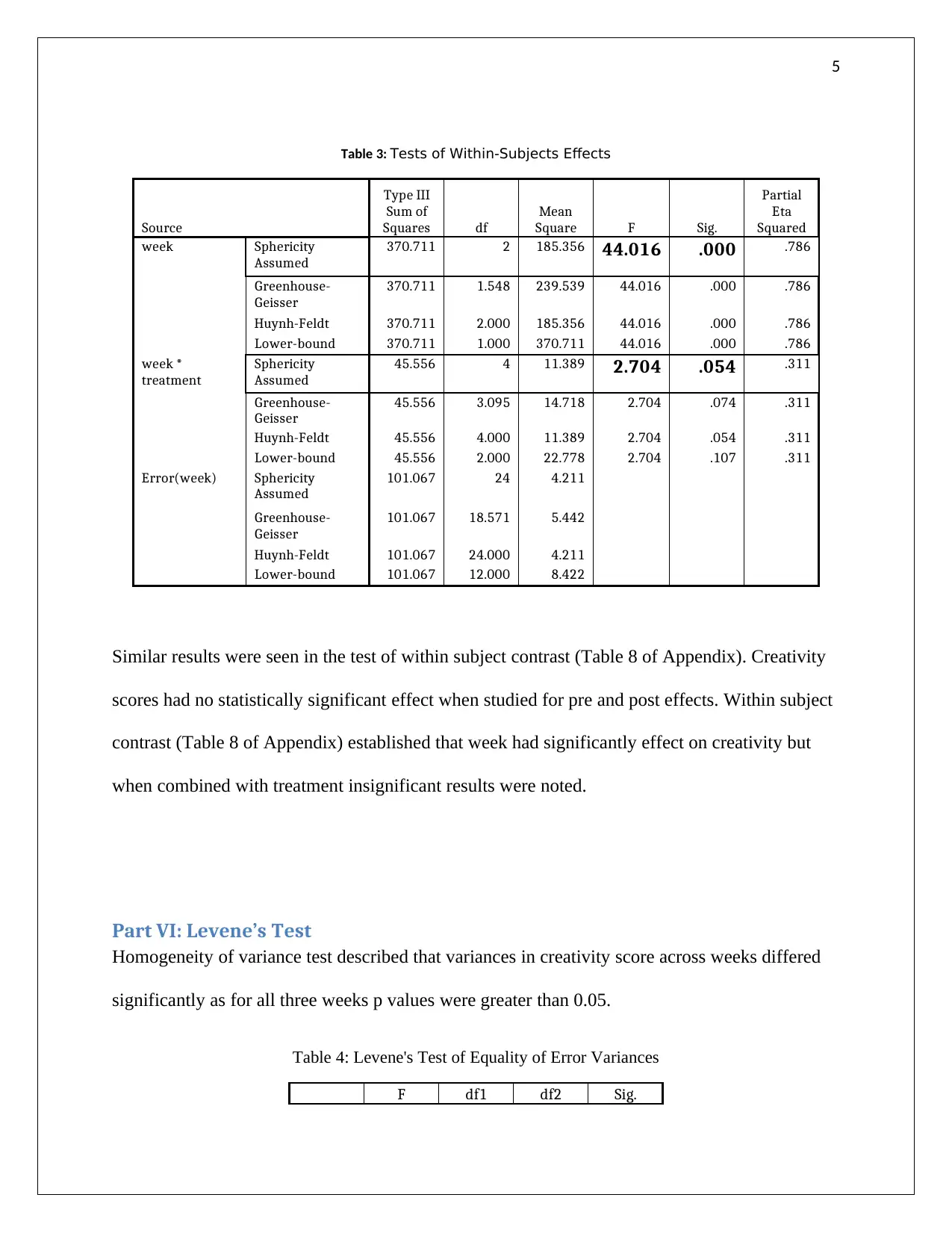
Table 3: Tests of Within-Subjects Effects
Source
Type III
Sum of
Squares df
Mean
Square F Sig.
Partial
Eta
Squared
week Sphericity
Assumed
370.711 2 185.356 44.016 .000 .786
Greenhouse-
Geisser
370.711 1.548 239.539 44.016 .000 .786
Huynh-Feldt 370.711 2.000 185.356 44.016 .000 .786
Lower-bound 370.711 1.000 370.711 44.016 .000 .786
week *
treatment
Sphericity
Assumed
45.556 4 11.389 2.704 .054 .311
Greenhouse-
Geisser
45.556 3.095 14.718 2.704 .074 .311
Huynh-Feldt 45.556 4.000 11.389 2.704 .054 .311
Lower-bound 45.556 2.000 22.778 2.704 .107 .311
Error(week) Sphericity
Assumed
101.067 24 4.211
Greenhouse-
Geisser
101.067 18.571 5.442
Huynh-Feldt 101.067 24.000 4.211
Lower-bound 101.067 12.000 8.422
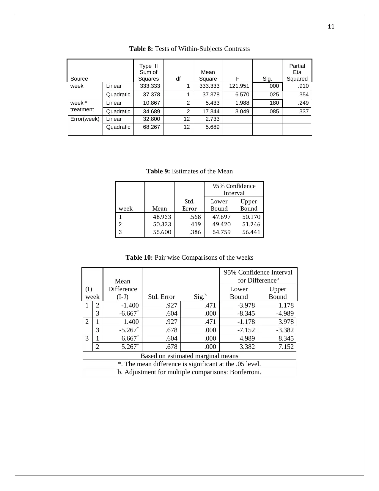
Similar results were seen in the test of within subject contrast (Table 8 of Appendix). Creativity
scores had no statistically significant effect when studied for pre and post effects. Within subject
contrast (Table 8 of Appendix) established that week had significantly effect on creativity but
when combined with treatment insignificant results were noted.
Part VI: Levene’s Test
Homogeneity of variance test described that variances in creativity score across weeks differed
significantly as for all three weeks p values were greater than 0.05.
Table 4: Levene's Test of Equality of Error Variances
F df1 df2 Sig.
Table 3: Tests of Within-Subjects Effects
Source
Type III
Sum of
Squares df
Mean
Square F Sig.
Partial
Eta
Squared
week Sphericity
Assumed
370.711 2 185.356 44.016 .000 .786
Greenhouse-
Geisser
370.711 1.548 239.539 44.016 .000 .786
Huynh-Feldt 370.711 2.000 185.356 44.016 .000 .786
Lower-bound 370.711 1.000 370.711 44.016 .000 .786
week *
treatment
Sphericity
Assumed
45.556 4 11.389 2.704 .054 .311
Greenhouse-
Geisser
45.556 3.095 14.718 2.704 .074 .311
Huynh-Feldt 45.556 4.000 11.389 2.704 .054 .311
Lower-bound 45.556 2.000 22.778 2.704 .107 .311
Error(week) Sphericity
Assumed
101.067 24 4.211
Greenhouse-
Geisser
101.067 18.571 5.442
Huynh-Feldt 101.067 24.000 4.211
Lower-bound 101.067 12.000 8.422
Similar results were seen in the test of within subject contrast (Table 8 of Appendix). Creativity
scores had no statistically significant effect when studied for pre and post effects. Within subject
contrast (Table 8 of Appendix) established that week had significantly effect on creativity but
when combined with treatment insignificant results were noted.
Part VI: Levene’s Test
Homogeneity of variance test described that variances in creativity score across weeks differed
significantly as for all three weeks p values were greater than 0.05.
Table 4: Levene's Test of Equality of Error Variances
F df1 df2 Sig.
6
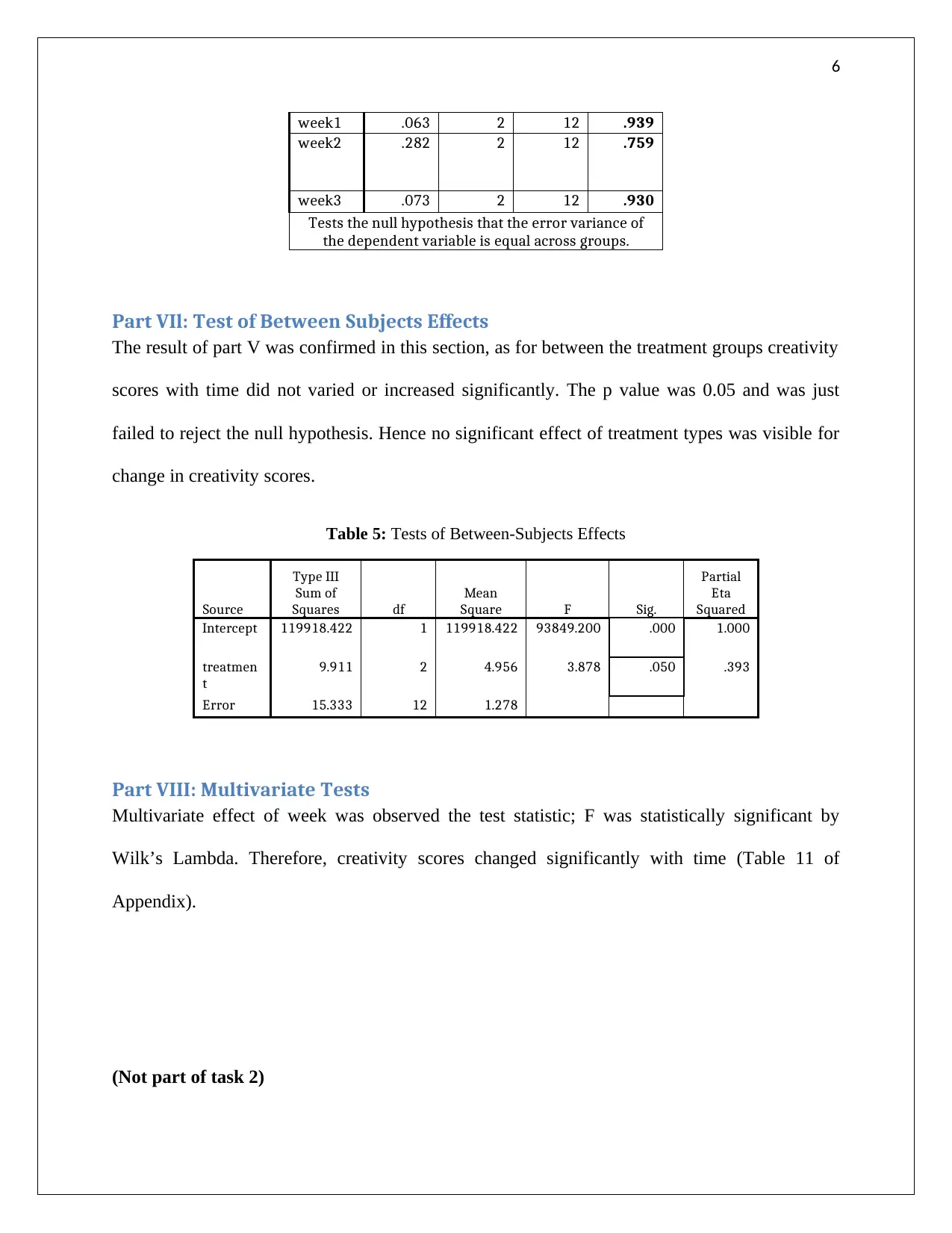
week1 .063 2 12 .939
week2 .282 2 12 .759
week3 .073 2 12 .930
Tests the null hypothesis that the error variance of
the dependent variable is equal across groups.
Part VIl: Test of Between Subjects Effects
The result of part V was confirmed in this section, as for between the treatment groups creativity
scores with time did not varied or increased significantly. The p value was 0.05 and was just
failed to reject the null hypothesis. Hence no significant effect of treatment types was visible for
change in creativity scores.
Table 5: Tests of Between-Subjects Effects
Source
Type III
Sum of
Squares df
Mean
Square F Sig.
Partial
Eta
Squared
Intercept 119918.422 1 119918.422 93849.200 .000 1.000
treatmen
t
9.911 2 4.956 3.878 .050 .393
Error 15.333 12 1.278
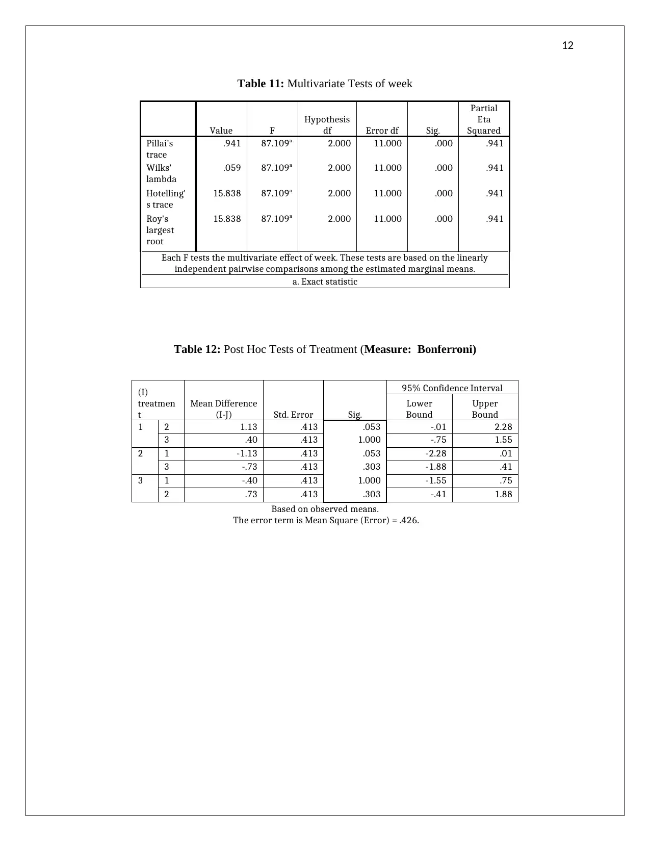
Part VIII: Multivariate Tests
Multivariate effect of week was observed the test statistic; F was statistically significant by
Wilk’s Lambda. Therefore, creativity scores changed significantly with time (Table 11 of
Appendix).
(Not part of task 2)
week1 .063 2 12 .939
week2 .282 2 12 .759
week3 .073 2 12 .930
Tests the null hypothesis that the error variance of
the dependent variable is equal across groups.
Part VIl: Test of Between Subjects Effects
The result of part V was confirmed in this section, as for between the treatment groups creativity
scores with time did not varied or increased significantly. The p value was 0.05 and was just
failed to reject the null hypothesis. Hence no significant effect of treatment types was visible for
change in creativity scores.
Table 5: Tests of Between-Subjects Effects
Source
Type III
Sum of
Squares df
Mean
Square F Sig.
Partial
Eta
Squared
Intercept 119918.422 1 119918.422 93849.200 .000 1.000
treatmen
t
9.911 2 4.956 3.878 .050 .393
Error 15.333 12 1.278
Part VIII: Multivariate Tests
Multivariate effect of week was observed the test statistic; F was statistically significant by
Wilk’s Lambda. Therefore, creativity scores changed significantly with time (Table 11 of
Appendix).
(Not part of task 2)
⊘ This is a preview!⊘
Do you want full access?
Subscribe today to unlock all pages.
Trusted by 1+ million students worldwide
7
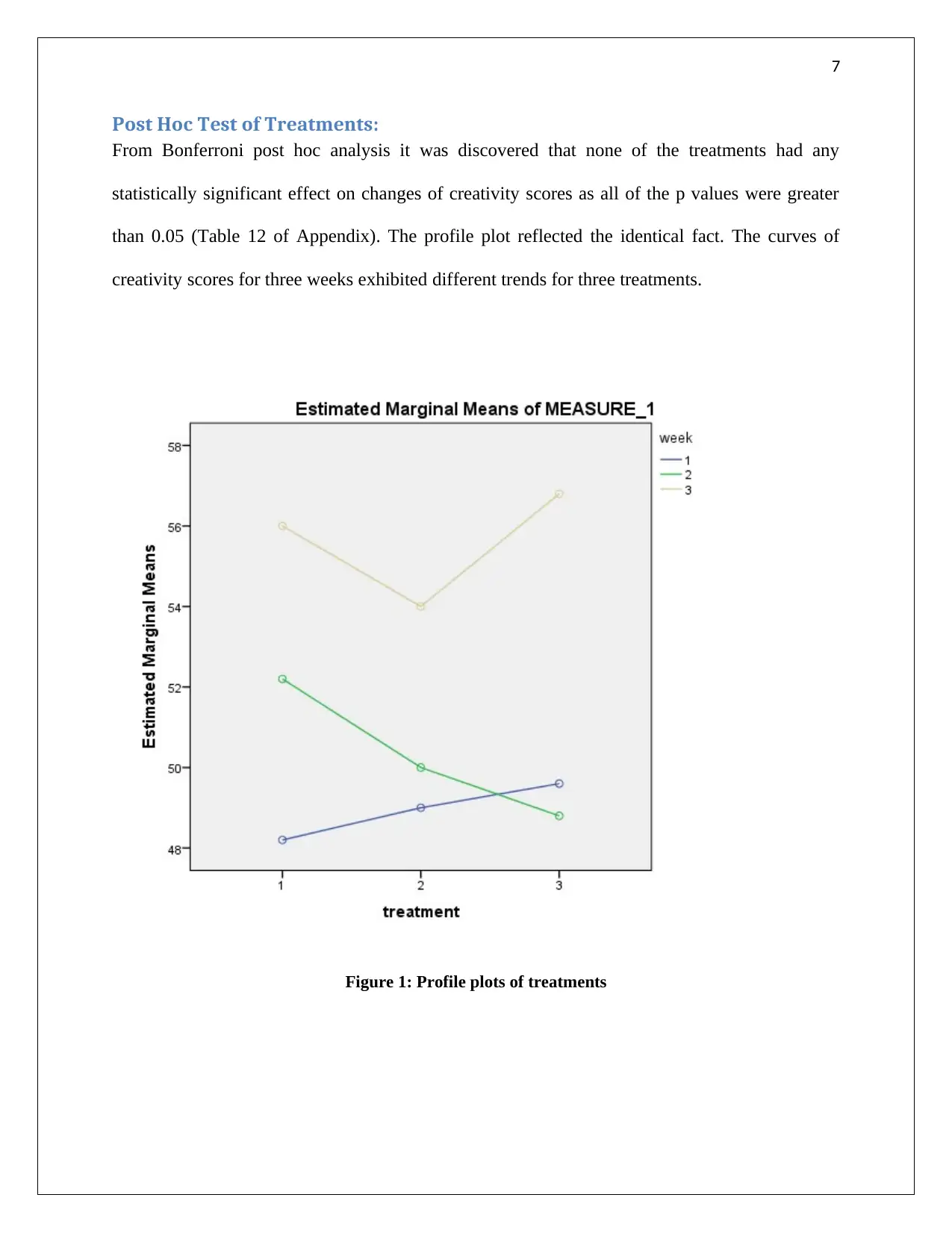
Post Hoc Test of Treatments:
From Bonferroni post hoc analysis it was discovered that none of the treatments had any
statistically significant effect on changes of creativity scores as all of the p values were greater
than 0.05 (Table 12 of Appendix). The profile plot reflected the identical fact. The curves of
creativity scores for three weeks exhibited different trends for three treatments.
Figure 1: Profile plots of treatments
Paraphrase This Document
Need a fresh take? Get an instant paraphrase of this document with our AI Paraphraser
8
Conclusion
Creativity scores significantly changed with time for each treatment. But treatments, when
considered for all three weeks did not have similar significant effects on the scores.
Divertimento Task
a) ANOVA uses categorical variable whereas ANCOVA uses categorical as well as interval
variable. ANOVA involves independent variable which is categorical in nature where
ANCOVA deals with metric independent and categorical variable. Independent variable
in ANOVA is considered as factor.
b) ANCOVA deals with group variation, that is, the variation of plate sizes is characterized
exclusively to body weight (in kg). The results will reveal the effect of body weight for
three different levels of plate sizes. The effect of metric independent variable of body
weight on consumption of food will be revealed (Jiang et al., 2016).
The interaction of body weight and categorical variable, plate size will disclose the group
variation of plate sizes to covariate of body weight. Correlation of body weight with plate
size weakens the ANCOVA results and increases the noise. The experiment, when
designed with three different size plates together on the same day and on different days
will help in decision making about the effectiveness of ANCOVA for the problem.
c) Study A: Age acts as an independent factor when used as a covariate in ANCOVA with
the four factors of the study. Hence, effect of the four factors on the dependent variable
(food wastage reduction) can be studied taking age as a covariate in the study.
Study B: Age does not act as an independent factor in this study. The three independent
factors have effect on age and correlation between them is evident. Hence ANCOVA
9
results, including age as cofactor will generate huge noise in the regression model (de
Vries et al., 2016).
Reference
de Vries, A. L., Steensma, T. D., Cohen-Kettenis, P. T., VanderLaan, D. P., & Zucker, K. J.
(2016). Poor peer relations predict parent-and self-reported behavioral and emotional
problems of adolescents with gender dysphoria: a cross-national, cross-clinic comparative
analysis. European child & adolescent psychiatry, 25(6), 579-588.
Jiang, F., Tian, L., Fu, H., Hasegawa, T., Pfeffer, M. A., & Wei, L. J. (2016). Robust alternatives
to ANCOVA for estimating the treatment effect via a randomized comparative study.
⊘ This is a preview!⊘
Do you want full access?
Subscribe today to unlock all pages.
Trusted by 1+ million students worldwide
10
Appendix
Table 6: Multivariate Test
Effect Value F
Hypothesi
s df Error df Sig.
Partial
Eta
Squared
week Pillai's
Trace
.941 87.109b 2.000 11.000 .000 .941
Wilks'
Lambda
.059 87.109b 2.000 11.000 .000 .941
Hotelling'
s Trace
15.838 87.109b 2.000 11.000 .000 .941
Roy's
Largest
Root
15.838 87.109b 2.000 11.000 .000 .941
week *
treatmen
t
Pillai's
Trace
.645 2.857 4.000 24.000 .046 .323
Wilks'
Lambda
.448 2.714b 4.000 22.000 .056 .330
Hotelling'
s Trace
1.022 2.556 4.000 20.000 .071 .338
Roy's
Largest
Root
.742 4.449c 2.000 12.000 .036 .426
a. Design: Intercept + treatment
Within Subjects Design: week
b. Exact statistic
c. The statistic is an upper bound on F that yields a lower bound on the significance level.
Table 7: Mauchly's Test of Sphericitya
Within
Subjects
Effect Mauchly's W
Approx.
Chi-
Square df Sig.
Epsilonb
Greenhouse-
Geisser
Huynh-
Feldt
Lower-
bound
week .708 3.803 2 .149 .774 1.000 .500
Tests the null hypothesis that the error covariance matrix of the orthonormalized transformed
dependent variables is proportional to an identity matrix.
a. Design: Intercept + treatment
Within Subjects Design: week
b. May be used to adjust the degrees of freedom for the averaged tests of significance. Corrected
tests are displayed in the Tests of Within-Subjects Effects table.
Paraphrase This Document
Need a fresh take? Get an instant paraphrase of this document with our AI Paraphraser
11
Table 8: Tests of Within-Subjects Contrasts
Source
Type III
Sum of
Squares df
Mean
Square F Sig.
Partial
Eta
Squared
week Linear 333.333 1 333.333 121.951 .000 .910
Quadratic 37.378 1 37.378 6.570 .025 .354
week *
treatment
Linear 10.867 2 5.433 1.988 .180 .249
Quadratic 34.689 2 17.344 3.049 .085 .337
Error(week) Linear 32.800 12 2.733
Quadratic 68.267 12 5.689
Table 9: Estimates of the Mean
week Mean
Std.
Error
95% Confidence
Interval
Lower
Bound
Upper
Bound
1 48.933 .568 47.697 50.170
2 50.333 .419 49.420 51.246
3 55.600 .386 54.759 56.441
Table 10: Pair wise Comparisons of the weeks
(I)
week
Mean
Difference
(I-J) Std. Error Sig.b
95% Confidence Interval
for Differenceb
Lower
Bound
Upper
Bound
1 2 -1.400 .927 .471 -3.978 1.178
3 -6.667* .604 .000 -8.345 -4.989
2 1 1.400 .927 .471 -1.178 3.978
3 -5.267* .678 .000 -7.152 -3.382
3 1 6.667* .604 .000 4.989 8.345
2 5.267* .678 .000 3.382 7.152
Based on estimated marginal means
*. The mean difference is significant at the .05 level.
b. Adjustment for multiple comparisons: Bonferroni.
12
Table 11: Multivariate Tests of week
Value F
Hypothesis
df Error df Sig.
Partial
Eta
Squared
Pillai's
trace
.941 87.109a 2.000 11.000 .000 .941
Wilks'
lambda
.059 87.109a 2.000 11.000 .000 .941
Hotelling'
s trace
15.838 87.109a 2.000 11.000 .000 .941
Roy's
largest
root
15.838 87.109a 2.000 11.000 .000 .941
Each F tests the multivariate effect of week. These tests are based on the linearly
independent pairwise comparisons among the estimated marginal means.
a. Exact statistic
Table 12: Post Hoc Tests of Treatment (Measure: Bonferroni)
(I)
treatmen
t
Mean Difference
(I-J) Std. Error Sig.
95% Confidence Interval
Lower
Bound
Upper
Bound
1 2 1.13 .413 .053 -.01 2.28
3 .40 .413 1.000 -.75 1.55
2 1 -1.13 .413 .053 -2.28 .01
3 -.73 .413 .303 -1.88 .41
3 1 -.40 .413 1.000 -1.55 .75
2 .73 .413 .303 -.41 1.88
Based on observed means.
The error term is Mean Square (Error) = .426.
⊘ This is a preview!⊘
Do you want full access?
Subscribe today to unlock all pages.
Trusted by 1+ million students worldwide
1 out of 12

Your All-in-One AI-Powered Toolkit for Academic Success.
+13062052269
info@desklib.com
Available 24*7 on WhatsApp / Email
![[object Object]](/_next/static/media/star-bottom.7253800d.svg)
Unlock your academic potential
Copyright © 2020–2026 A2Z Services. All Rights Reserved. Developed and managed by ZUCOL.