Quantitative Techniques in Business Analysis - Semester 1 Report
VerifiedAdded on 2022/12/19
|13
|2352
|45
Report
AI Summary
This report, focusing on quantitative techniques in business, systematically analyzes data to derive meaningful insights for decision-making. It employs various methods, including regression and correlation analysis, to examine the relationships between income levels, education, and work experience. The report presents findings through graphical representations and statistical summaries, such as ANOVA tables and regression statistics, to assess the impact of factors like education, experience, and previous jobs on income. The analysis reveals positive correlations between income and both education and work experience, while highlighting the importance of these variables for strategic planning. The report concludes with recommendations for personnel and recruitment companies to develop models considering these relationships to improve outcomes.

Quantitative Techniques
in Business
1
in Business
1
Paraphrase This Document
Need a fresh take? Get an instant paraphrase of this document with our AI Paraphraser
Contents
Contents...........................................................................................................................................2
Introduction......................................................................................................................................3
TASK A...........................................................................................................................................3
TASK 1........................................................................................................................................3
TASK 2........................................................................................................................................4
TASK 3........................................................................................................................................6
Conclusion and Recommendations................................................................................................10
TASK B.........................................................................................................................................11
This part has been covered in PPT............................................................................................11
REFERENCES..............................................................................................................................12
2
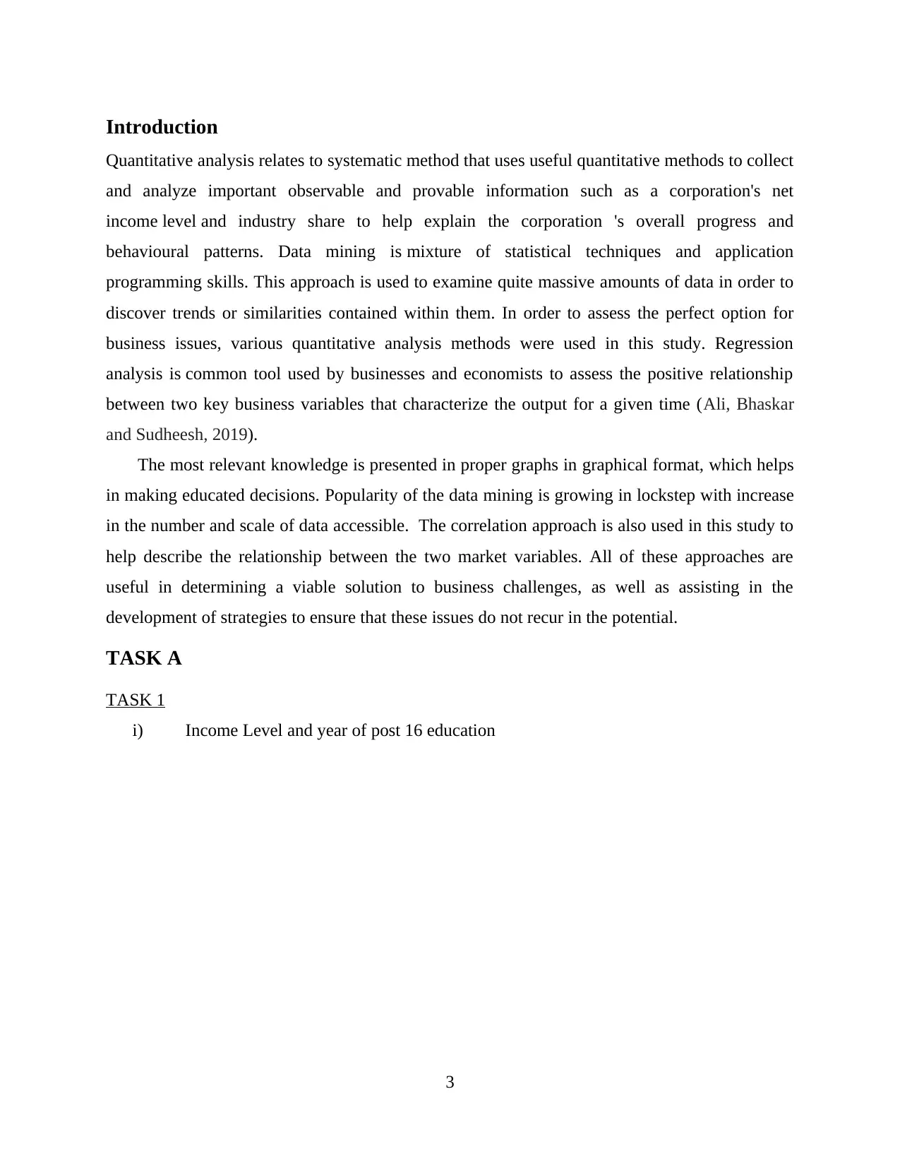
Introduction
Quantitative analysis relates to systematic method that uses useful quantitative methods to collect
and analyze important observable and provable information such as a corporation's net
income level and industry share to help explain the corporation 's overall progress and
behavioural patterns. Data mining is mixture of statistical techniques and application
programming skills. This approach is used to examine quite massive amounts of data in order to
discover trends or similarities contained within them. In order to assess the perfect option for
business issues, various quantitative analysis methods were used in this study. Regression
analysis is common tool used by businesses and economists to assess the positive relationship
between two key business variables that characterize the output for a given time (Ali, Bhaskar
and Sudheesh, 2019).
The most relevant knowledge is presented in proper graphs in graphical format, which helps
in making educated decisions. Popularity of the data mining is growing in lockstep with increase
in the number and scale of data accessible. The correlation approach is also used in this study to
help describe the relationship between the two market variables. All of these approaches are
useful in determining a viable solution to business challenges, as well as assisting in the
development of strategies to ensure that these issues do not recur in the potential.
TASK A
TASK 1
i) Income Level and year of post 16 education
3
⊘ This is a preview!⊘
Do you want full access?
Subscribe today to unlock all pages.
Trusted by 1+ million students worldwide
1 2 3 4 5 6 7 8 9 10 11 12 13
0
5
10
15
20
25
30
35
40
45
15
20
17
9
18
24
37
24
19 21
39
24 22
2
5 5
2
5 7
10
5 6
2
7 8
5
Income level Years of post-16 education
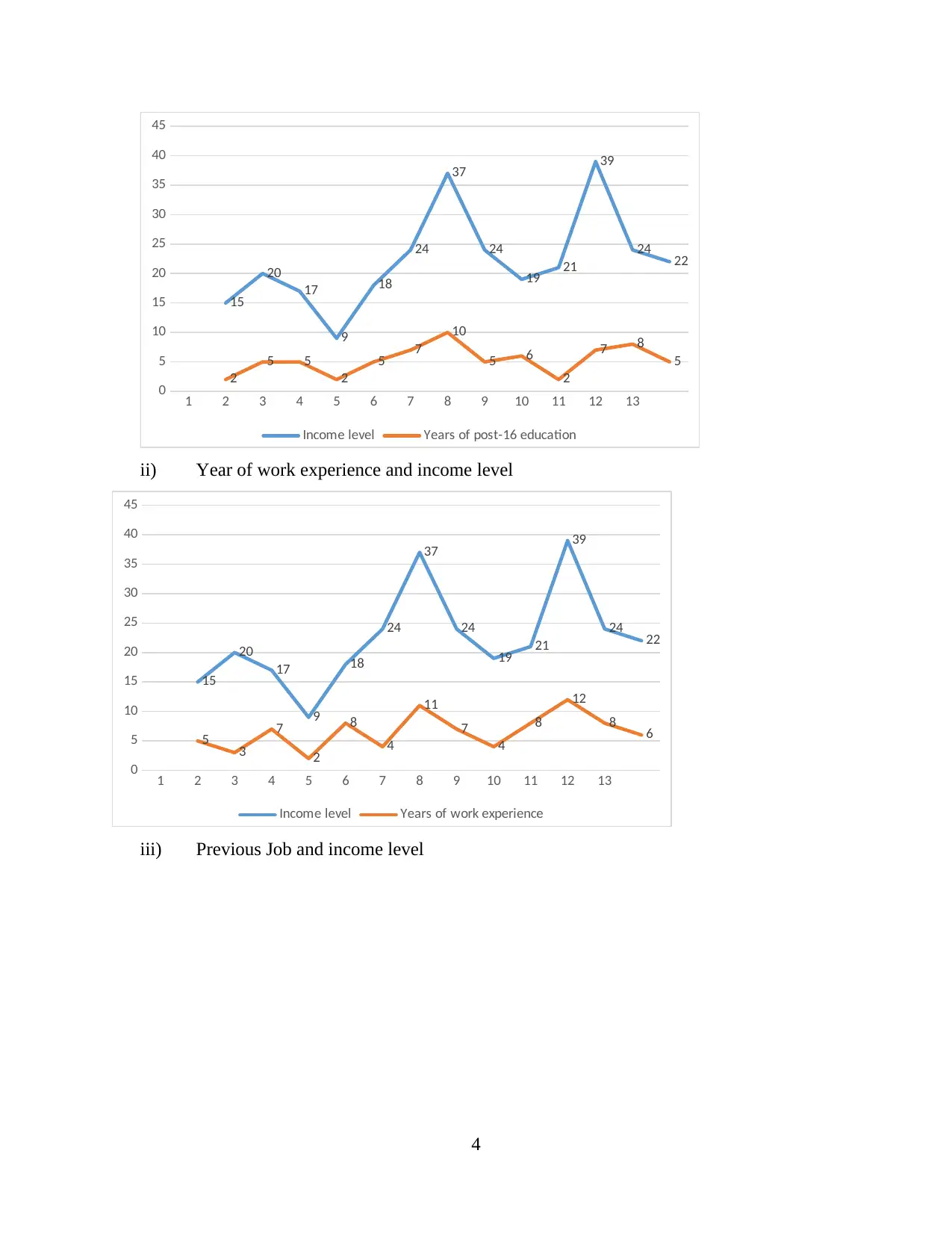
ii) Year of work experience and income level
1 2 3 4 5 6 7 8 9 10 11 12 13
0
5
10
15
20
25
30
35
40
45
15
20
17
9
18
24
37
24
19 21
39
24 22
5 3
7
2
8
4
11
7
4
8
12
8 6
Income level Years of work experience
iii) Previous Job and income level
4
0
5
10
15
20
25
30
35
40
45
15
20
17
9
18
24
37
24
19 21
39
24 22
2
5 5
2
5 7
10
5 6
2
7 8
5
Income level Years of post-16 education
ii) Year of work experience and income level
1 2 3 4 5 6 7 8 9 10 11 12 13
0
5
10
15
20
25
30
35
40
45
15
20
17
9
18
24
37
24
19 21
39
24 22
5 3
7
2
8
4
11
7
4
8
12
8 6
Income level Years of work experience
iii) Previous Job and income level
4
Paraphrase This Document
Need a fresh take? Get an instant paraphrase of this document with our AI Paraphraser
1 2 3 4 5 6 7 8 9 10 11 12 13
0
5
10
15
20
25
30
35
40
45
15
20
17
9
18
24
37
24
19 21
39
24 22
0 1 2 0 2 3 2 1 0
4 2 1 2
Income level Number of previous jobs
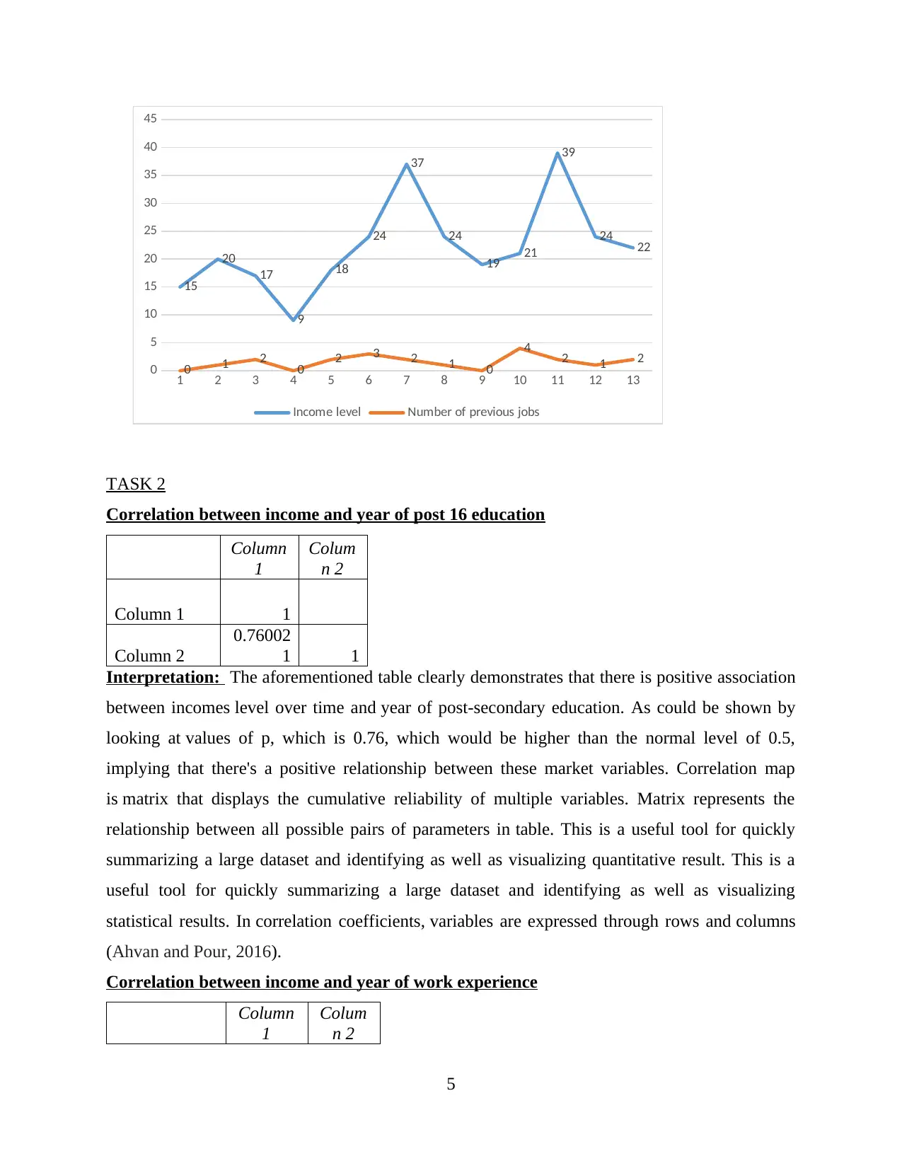
TASK 2
Correlation between income and year of post 16 education
Column
1
Colum
n 2
Column 1 1
Column 2
0.76002
1 1
Interpretation: The aforementioned table clearly demonstrates that there is positive association
between incomes level over time and year of post-secondary education. As could be shown by
looking at values of p, which is 0.76, which would be higher than the normal level of 0.5,
implying that there's a positive relationship between these market variables. Correlation map
is matrix that displays the cumulative reliability of multiple variables. Matrix represents the
relationship between all possible pairs of parameters in table. This is a useful tool for quickly
summarizing a large dataset and identifying as well as visualizing quantitative result. This is a
useful tool for quickly summarizing a large dataset and identifying as well as visualizing
statistical results. In correlation coefficients, variables are expressed through rows and columns
(Ahvan and Pour, 2016).
Correlation between income and year of work experience
Column
1
Colum
n 2
5
0
5
10
15
20
25
30
35
40
45
15
20
17
9
18
24
37
24
19 21
39
24 22
0 1 2 0 2 3 2 1 0
4 2 1 2
Income level Number of previous jobs
TASK 2
Correlation between income and year of post 16 education
Column
1
Colum
n 2
Column 1 1
Column 2
0.76002
1 1
Interpretation: The aforementioned table clearly demonstrates that there is positive association
between incomes level over time and year of post-secondary education. As could be shown by
looking at values of p, which is 0.76, which would be higher than the normal level of 0.5,
implying that there's a positive relationship between these market variables. Correlation map
is matrix that displays the cumulative reliability of multiple variables. Matrix represents the
relationship between all possible pairs of parameters in table. This is a useful tool for quickly
summarizing a large dataset and identifying as well as visualizing quantitative result. This is a
useful tool for quickly summarizing a large dataset and identifying as well as visualizing
statistical results. In correlation coefficients, variables are expressed through rows and columns
(Ahvan and Pour, 2016).
Correlation between income and year of work experience
Column
1
Colum
n 2
5
Column 1 1
Column 2 0.805222 1
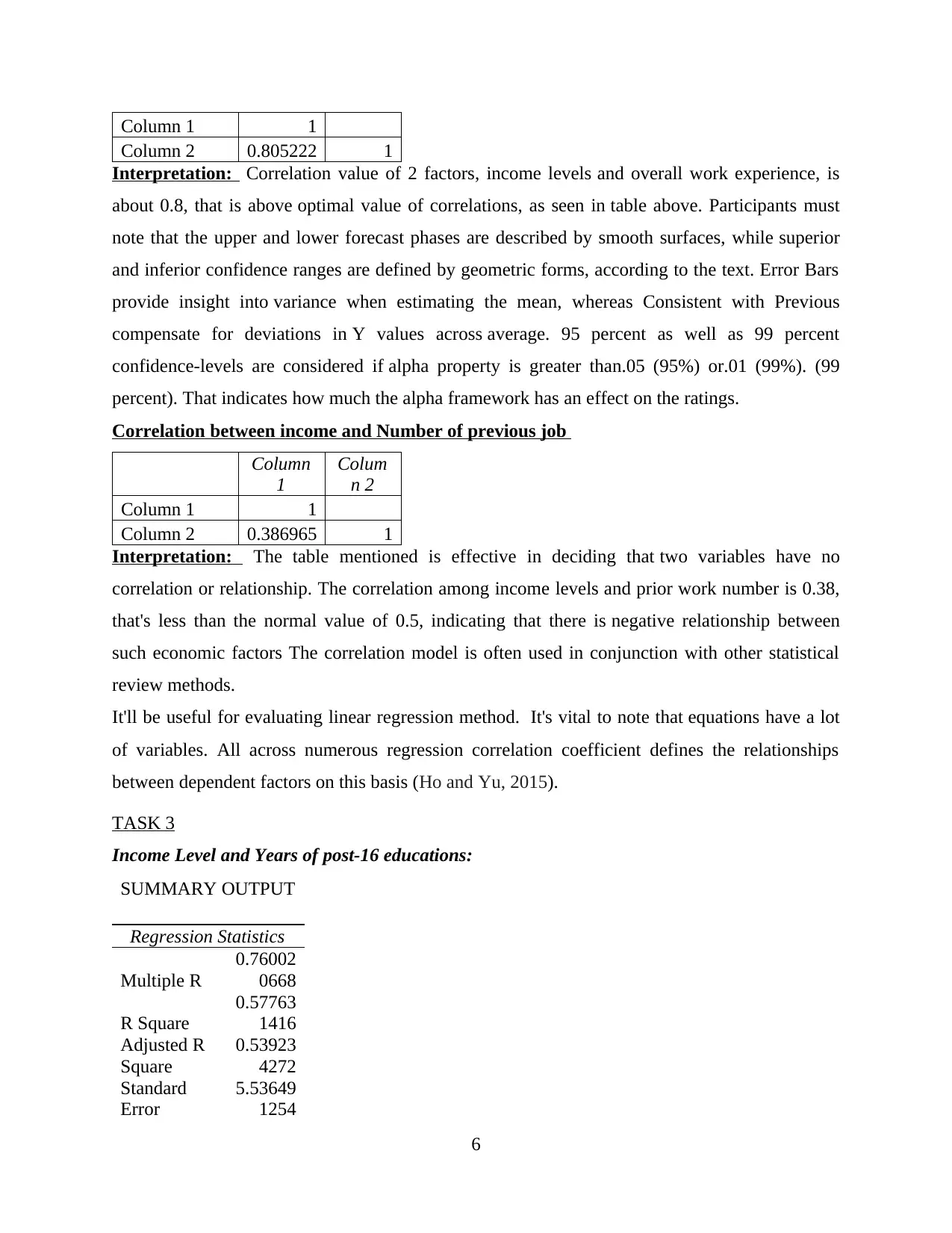
Interpretation: Correlation value of 2 factors, income levels and overall work experience, is
about 0.8, that is above optimal value of correlations, as seen in table above. Participants must
note that the upper and lower forecast phases are described by smooth surfaces, while superior
and inferior confidence ranges are defined by geometric forms, according to the text. Error Bars
provide insight into variance when estimating the mean, whereas Consistent with Previous
compensate for deviations in Y values across average. 95 percent as well as 99 percent
confidence-levels are considered if alpha property is greater than.05 (95%) or.01 (99%). (99
percent). That indicates how much the alpha framework has an effect on the ratings.
Correlation between income and Number of previous job
Column
1
Colum
n 2
Column 1 1
Column 2 0.386965 1
Interpretation: The table mentioned is effective in deciding that two variables have no
correlation or relationship. The correlation among income levels and prior work number is 0.38,
that's less than the normal value of 0.5, indicating that there is negative relationship between
such economic factors The correlation model is often used in conjunction with other statistical
review methods.
It'll be useful for evaluating linear regression method. It's vital to note that equations have a lot
of variables. All across numerous regression correlation coefficient defines the relationships
between dependent factors on this basis (Ho and Yu, 2015).
TASK 3
Income Level and Years of post-16 educations:
SUMMARY OUTPUT
Regression Statistics
Multiple R
0.76002
0668
R Square
0.57763
1416
Adjusted R
Square
0.53923
4272
Standard
Error
5.53649
1254
6
Column 2 0.805222 1
Interpretation: Correlation value of 2 factors, income levels and overall work experience, is
about 0.8, that is above optimal value of correlations, as seen in table above. Participants must
note that the upper and lower forecast phases are described by smooth surfaces, while superior
and inferior confidence ranges are defined by geometric forms, according to the text. Error Bars
provide insight into variance when estimating the mean, whereas Consistent with Previous
compensate for deviations in Y values across average. 95 percent as well as 99 percent
confidence-levels are considered if alpha property is greater than.05 (95%) or.01 (99%). (99
percent). That indicates how much the alpha framework has an effect on the ratings.
Correlation between income and Number of previous job
Column
1
Colum
n 2
Column 1 1
Column 2 0.386965 1
Interpretation: The table mentioned is effective in deciding that two variables have no
correlation or relationship. The correlation among income levels and prior work number is 0.38,
that's less than the normal value of 0.5, indicating that there is negative relationship between
such economic factors The correlation model is often used in conjunction with other statistical
review methods.
It'll be useful for evaluating linear regression method. It's vital to note that equations have a lot
of variables. All across numerous regression correlation coefficient defines the relationships
between dependent factors on this basis (Ho and Yu, 2015).
TASK 3
Income Level and Years of post-16 educations:
SUMMARY OUTPUT
Regression Statistics
Multiple R
0.76002
0668
R Square
0.57763
1416
Adjusted R
Square
0.53923
4272
Standard
Error
5.53649
1254
6
⊘ This is a preview!⊘
Do you want full access?
Subscribe today to unlock all pages.
Trusted by 1+ million students worldwide
Observation
s 13
ANOVA
df SS MS F
Signific
ance F
Regression 1 461.1276
461.1
276
15.04
36 0.00257
Residual 11 337.1801
30.65
274
Total 12 798.3077
Coeffici
ents
Standard
Error t Stat
P-
value
Lower
95%
Upper
95%
Lower
95.0%
Upper
95.0%
Intercept
8.48657
7181 3.861984
2.197
466
0.050
308
-
0.01359
16.986
75
-
0.01359
16.9867
5
X Variable
1
2.58948
5459 0.667633
3.878
608
0.002
57
1.12003
6
4.0589
35
1.12003
6
4.05893
5
RESIDUAL
OUTPUT
Observation Predicted Y Residuals
Standard
Residuals
1 13.6655481 1.334452 0.251746
2 21.43400447 -1.434 -0.27053
3 21.43400447 -4.434 -0.83648
4 13.6655481 -4.66555 -0.88016
5 21.43400447 -3.434 -0.64783
6 26.61297539 -2.61298 -0.49294
7 34.38143177 2.618568 0.493996
8 21.43400447 2.565996 0.484078
9 24.02348993 -5.02349 -0.94769
10 13.6655481 7.334452 1.383653
11 26.61297539 12.38702 2.336828
12 29.20246085 -5.20246 -0.98145
13 21.43400447 0.565996 0.106776
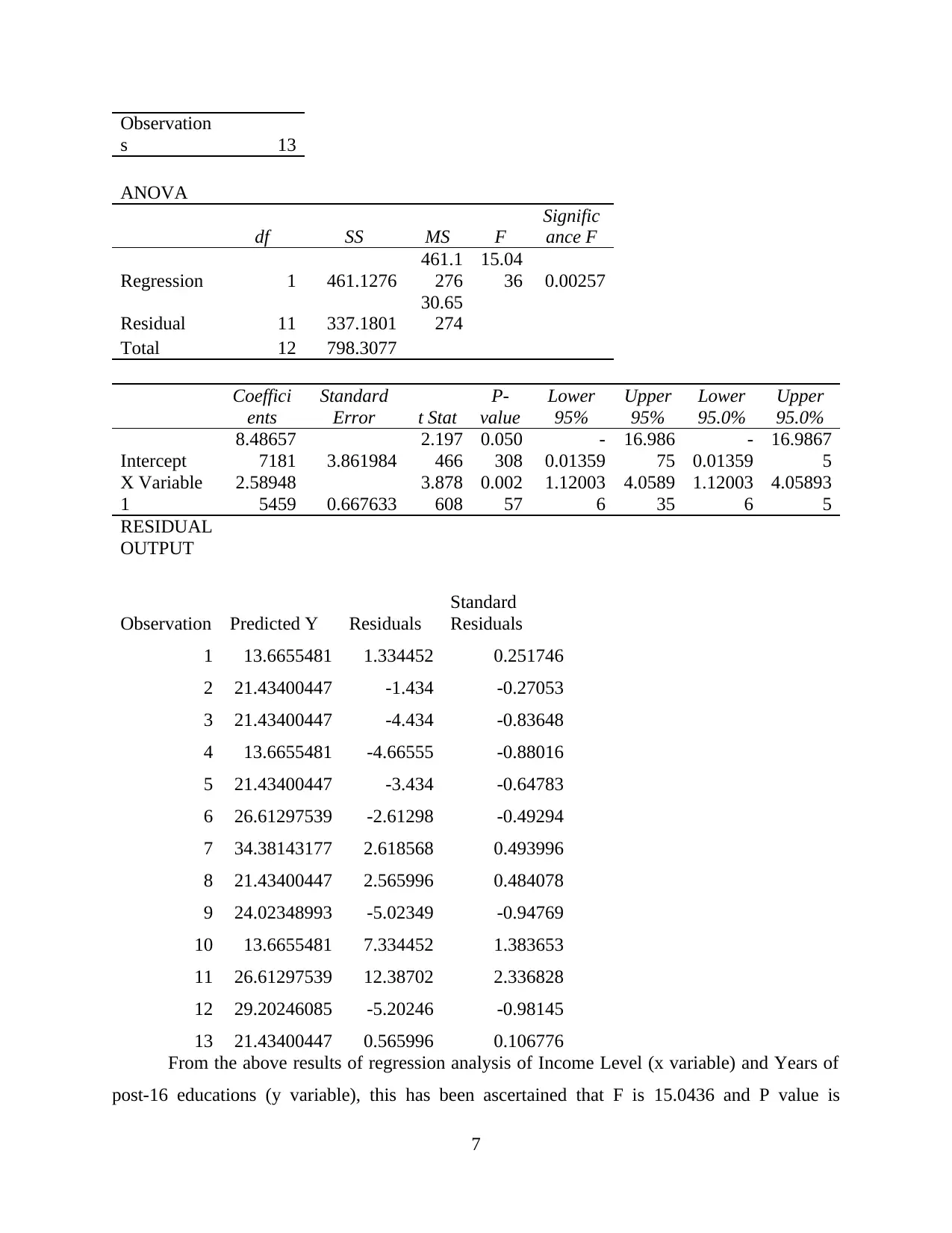
From the above results of regression analysis of Income Level (x variable) and Years of
post-16 educations (y variable), this has been ascertained that F is 15.0436 and P value is
7
s 13
ANOVA
df SS MS F
Signific
ance F
Regression 1 461.1276
461.1
276
15.04
36 0.00257
Residual 11 337.1801
30.65
274
Total 12 798.3077
Coeffici
ents
Standard
Error t Stat
P-
value
Lower
95%
Upper
95%
Lower
95.0%
Upper
95.0%
Intercept
8.48657
7181 3.861984
2.197
466
0.050
308
-
0.01359
16.986
75
-
0.01359
16.9867
5
X Variable
1
2.58948
5459 0.667633
3.878
608
0.002
57
1.12003
6
4.0589
35
1.12003
6
4.05893
5
RESIDUAL
OUTPUT
Observation Predicted Y Residuals
Standard
Residuals
1 13.6655481 1.334452 0.251746
2 21.43400447 -1.434 -0.27053
3 21.43400447 -4.434 -0.83648
4 13.6655481 -4.66555 -0.88016
5 21.43400447 -3.434 -0.64783
6 26.61297539 -2.61298 -0.49294
7 34.38143177 2.618568 0.493996
8 21.43400447 2.565996 0.484078
9 24.02348993 -5.02349 -0.94769
10 13.6655481 7.334452 1.383653
11 26.61297539 12.38702 2.336828
12 29.20246085 -5.20246 -0.98145
13 21.43400447 0.565996 0.106776
From the above results of regression analysis of Income Level (x variable) and Years of
post-16 educations (y variable), this has been ascertained that F is 15.0436 and P value is
7
Paraphrase This Document
Need a fresh take? Get an instant paraphrase of this document with our AI Paraphraser
0.050308. Since F value is greater than 1, this indicates that variation between group means are
more than expected. While the p-value is above significance level, which indicates that there are
not enough evidences to reject null hypothesis of which population means are equal (Ho and Yu,
2015).
Income level and Years of work experience:
SUMMARY
OUTPUT
Regression Statistics
Multiple R
0.76002
0668
R Square
0.57763
1416
Adjusted R
Square
0.53923
4272
Standard
Error
5.53649
1254
Observatio
ns 13
ANOVA
df SS MS F
Significa
nce F
Regression 1 461.1276
461.1
276
15.04
36 0.00257
Residual 11 337.1801
30.65
274
Total 12 798.3077
Coeffici
ents
Standard
Error t Stat
P-
value
Lower
95%
Upper
95%
Lower
95.0%
Upper
95.0%
Intercept
8.48657
7181 3.861984
2.197
466
0.050
308 -0.01359
16.986
75
-
0.01359
16.9867
5
X Variable
1
2.58948
5459 0.667633
3.878
608
0.002
57 1.120036
4.0589
35
1.12003
6
4.05893
5
RESIDUAL OUTPUT
Observatio
n Predicted Y
Residual
s
Standard
Residuals
1 13.6655481
1.33445
2 0.251746
8
2 21.43400447 -1.434 -0.27053
3 21.43400447 -4.434 -0.83648
4 13.6655481 -4.66555 -0.88016
5 21.43400447 -3.434 -0.64783
6 26.61297539 -2.61298 -0.49294
7 34.38143177
2.61856
8 0.493996
8 21.43400447
2.56599
6 0.484078
9 24.02348993 -5.02349 -0.94769
10 13.6655481
7.33445
2 1.383653
11 26.61297539
12.3870
2 2.336828
12 29.20246085 -5.20246 -0.98145
13 21.43400447
0.56599
6 0.106776
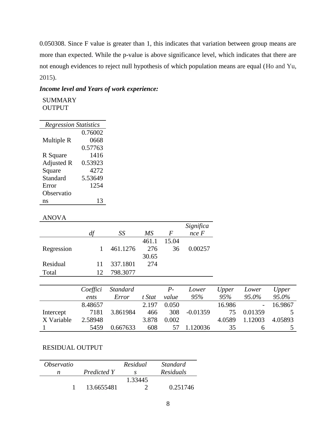
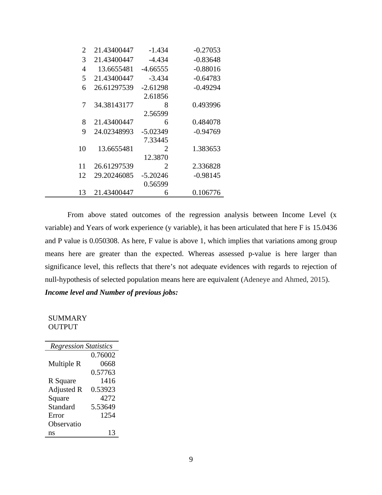
From above stated outcomes of the regression analysis between Income Level (x
variable) and Years of work experience (y variable), it has been articulated that here F is 15.0436
and P value is 0.050308. As here, F value is above 1, which implies that variations among group
means here are greater than the expected. Whereas assessed p-value is here larger than
significance level, this reflects that there’s not adequate evidences with regards to rejection of
null-hypothesis of selected population means here are equivalent (Adeneye and Ahmed, 2015).
Income level and Number of previous jobs:
SUMMARY
OUTPUT
Regression Statistics
Multiple R
0.76002
0668
R Square
0.57763
1416
Adjusted R
Square
0.53923
4272
Standard
Error
5.53649
1254
Observatio
ns 13
9
3 21.43400447 -4.434 -0.83648
4 13.6655481 -4.66555 -0.88016
5 21.43400447 -3.434 -0.64783
6 26.61297539 -2.61298 -0.49294
7 34.38143177
2.61856
8 0.493996
8 21.43400447
2.56599
6 0.484078
9 24.02348993 -5.02349 -0.94769
10 13.6655481
7.33445
2 1.383653
11 26.61297539
12.3870
2 2.336828
12 29.20246085 -5.20246 -0.98145
13 21.43400447
0.56599
6 0.106776
From above stated outcomes of the regression analysis between Income Level (x
variable) and Years of work experience (y variable), it has been articulated that here F is 15.0436
and P value is 0.050308. As here, F value is above 1, which implies that variations among group
means here are greater than the expected. Whereas assessed p-value is here larger than
significance level, this reflects that there’s not adequate evidences with regards to rejection of
null-hypothesis of selected population means here are equivalent (Adeneye and Ahmed, 2015).
Income level and Number of previous jobs:
SUMMARY
OUTPUT
Regression Statistics
Multiple R
0.76002
0668
R Square
0.57763
1416
Adjusted R
Square
0.53923
4272
Standard
Error
5.53649
1254
Observatio
ns 13
9
⊘ This is a preview!⊘
Do you want full access?
Subscribe today to unlock all pages.
Trusted by 1+ million students worldwide
ANOVA
df SS MS F
Signific
ance F
Regression 1
461.1276
028
461.127
6028
15.04
36 0.00257
Residual 11
337.1800
895
30.6527
3541
Total 12
798.3076
923
Coeffici
ents
Standard
Error t Stat
P-
value
Lower
95%
Upper
95%
Lower
95.0%
Upper
95.0%
Intercept
8.48657
7181
3.861984
152
2.19746
5564
0.050
308 -0.01359
16.986
75
-
0.01359
16.9867
5
X Variable
1
2.58948
5459
0.667632
6
3.87860
8471
0.002
57
1.12003
6
4.0589
35
1.12003
6
4.05893
5
RESIDUAL OUTPUT
Observatio
n Predicted Y Residuals
Standard
Residuals
1 13.6655481
1.33445190
2 0.251746005
2
21.4340044
7
-
1.43400447
4 -0.270526721
3
21.4340044
7
-
4.43400447
4 -0.836480439
4 13.6655481
-
4.66554809
8 -0.88016143
5
21.4340044
7
-
3.43400447
4 -0.647829199
6
26.6129753
9
-
2.61297539
1 -0.492941046
7
34.3814317
7
2.61856823
3 0.493996142
8
21.4340044
7
2.56599552
6 0.484078236
9
24.0234899
3
-
5.02348993
3 -0.947687601
10
Paraphrase This Document
Need a fresh take? Get an instant paraphrase of this document with our AI Paraphraser
10 13.6655481
7.33445190
2 1.38365344
11
26.6129753
9
12.3870246
1 2.336827542
12
29.2024608
5 -5.20246085 -0.981450686
13
21.4340044
7
0.56599552
6 0.106775757
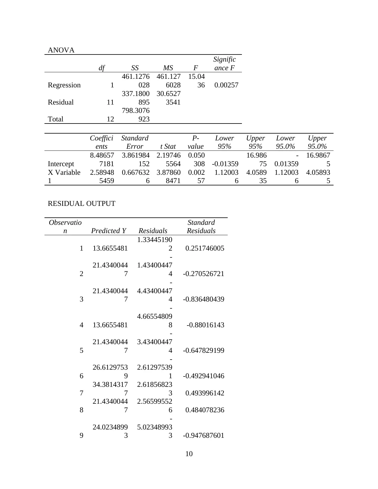
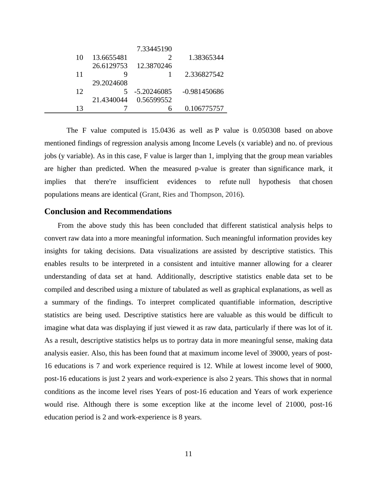
The F value computed is 15.0436 as well as P value is 0.050308 based on above
mentioned findings of regression analysis among Income Levels (x variable) and no. of previous
jobs (y variable). As in this case, F value is larger than 1, implying that the group mean variables
are higher than predicted. When the measured p-value is greater than significance mark, it
implies that there're insufficient evidences to refute null hypothesis that chosen
populations means are identical (Grant, Ries and Thompson, 2016).
Conclusion and Recommendations
From the above study this has been concluded that different statistical analysis helps to
convert raw data into a more meaningful information. Such meaningful information provides key
insights for taking decisions. Data visualizations are assisted by descriptive statistics. This
enables results to be interpreted in a consistent and intuitive manner allowing for a clearer
understanding of data set at hand. Additionally, descriptive statistics enable data set to be
compiled and described using a mixture of tabulated as well as graphical explanations, as well as
a summary of the findings. To interpret complicated quantifiable information, descriptive
statistics are being used. Descriptive statistics here are valuable as this would be difficult to
imagine what data was displaying if just viewed it as raw data, particularly if there was lot of it.
As a result, descriptive statistics helps us to portray data in more meaningful sense, making data
analysis easier. Also, this has been found that at maximum income level of 39000, years of post-
16 educations is 7 and work experience required is 12. While at lowest income level of 9000,
post-16 educations is just 2 years and work-experience is also 2 years. This shows that in normal
conditions as the income level rises Years of post-16 education and Years of work experience
would rise. Although there is some exception like at the income level of 21000, post-16
education period is 2 and work-experience is 8 years.
11
7.33445190
2 1.38365344
11
26.6129753
9
12.3870246
1 2.336827542
12
29.2024608
5 -5.20246085 -0.981450686
13
21.4340044
7
0.56599552
6 0.106775757
The F value computed is 15.0436 as well as P value is 0.050308 based on above
mentioned findings of regression analysis among Income Levels (x variable) and no. of previous
jobs (y variable). As in this case, F value is larger than 1, implying that the group mean variables
are higher than predicted. When the measured p-value is greater than significance mark, it
implies that there're insufficient evidences to refute null hypothesis that chosen
populations means are identical (Grant, Ries and Thompson, 2016).
Conclusion and Recommendations
From the above study this has been concluded that different statistical analysis helps to
convert raw data into a more meaningful information. Such meaningful information provides key
insights for taking decisions. Data visualizations are assisted by descriptive statistics. This
enables results to be interpreted in a consistent and intuitive manner allowing for a clearer
understanding of data set at hand. Additionally, descriptive statistics enable data set to be
compiled and described using a mixture of tabulated as well as graphical explanations, as well as
a summary of the findings. To interpret complicated quantifiable information, descriptive
statistics are being used. Descriptive statistics here are valuable as this would be difficult to
imagine what data was displaying if just viewed it as raw data, particularly if there was lot of it.
As a result, descriptive statistics helps us to portray data in more meaningful sense, making data
analysis easier. Also, this has been found that at maximum income level of 39000, years of post-
16 educations is 7 and work experience required is 12. While at lowest income level of 9000,
post-16 educations is just 2 years and work-experience is also 2 years. This shows that in normal
conditions as the income level rises Years of post-16 education and Years of work experience
would rise. Although there is some exception like at the income level of 21000, post-16
education period is 2 and work-experience is 8 years.
11
Here based on above findings and results this has been recommended to personnel and
recruitment company to prepare a model by considering above trends and results. Significance
level of education, experience and number of previous jobs is sold evidence that these factors are
dependent and have significant relation with Income levels. Also correlation analysis suggests
that there is direct relation between income level with education, experience and no. of jobs.
Thus company should prepare model while considering relation among these variables for better
outcomes.
TASK B
This part has been covered in PPT.
12
⊘ This is a preview!⊘
Do you want full access?
Subscribe today to unlock all pages.
Trusted by 1+ million students worldwide
1 out of 13
Related Documents


Your All-in-One AI-Powered Toolkit for Academic Success.
+13062052269
info@desklib.com
Available 24*7 on WhatsApp / Email
![[object Object]](/_next/static/media/star-bottom.7253800d.svg)
Unlock your academic potential
Copyright © 2020–2026 A2Z Services. All Rights Reserved. Developed and managed by ZUCOL.