Data Analysis in R: Descriptive Stats, Histograms, and Relationships

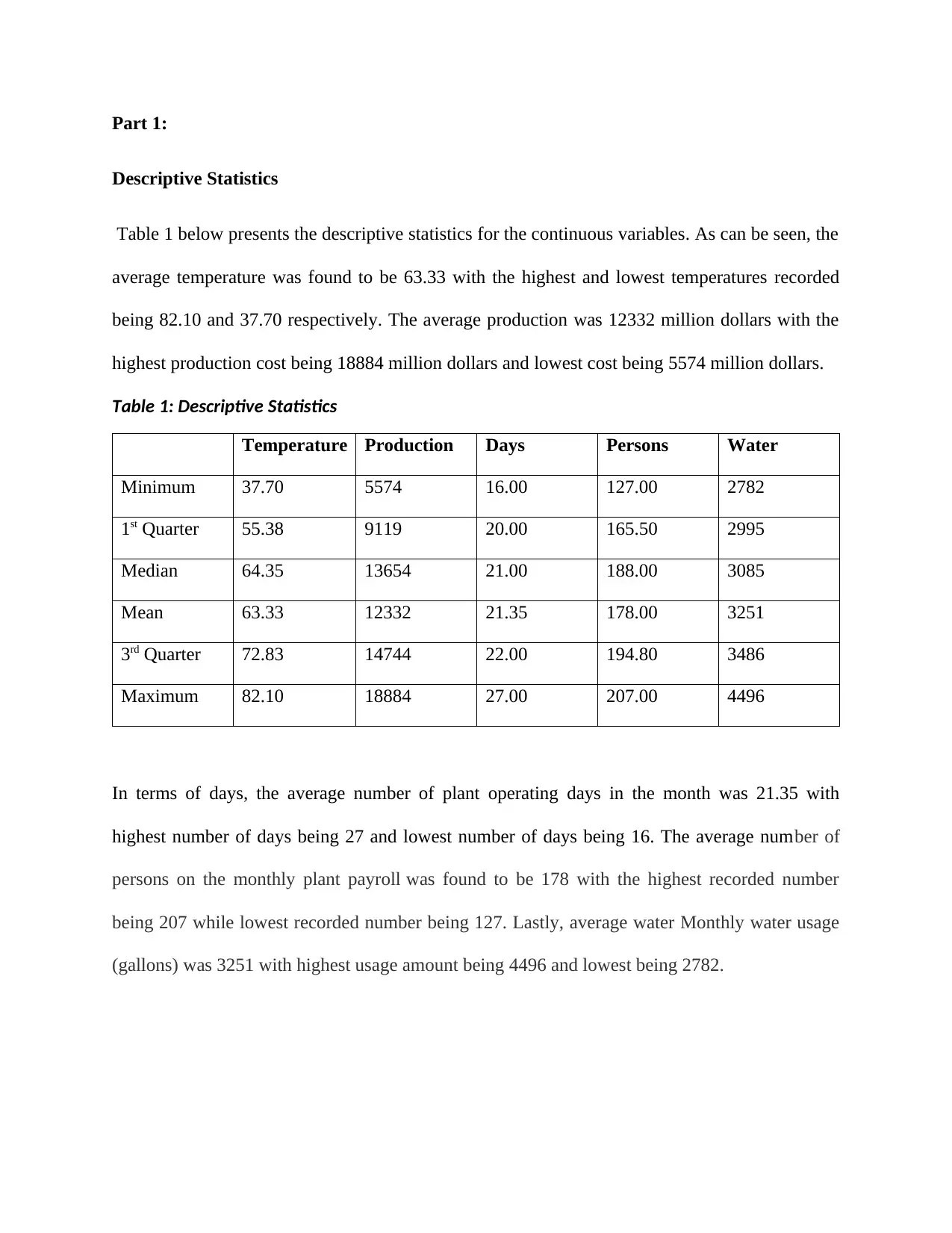
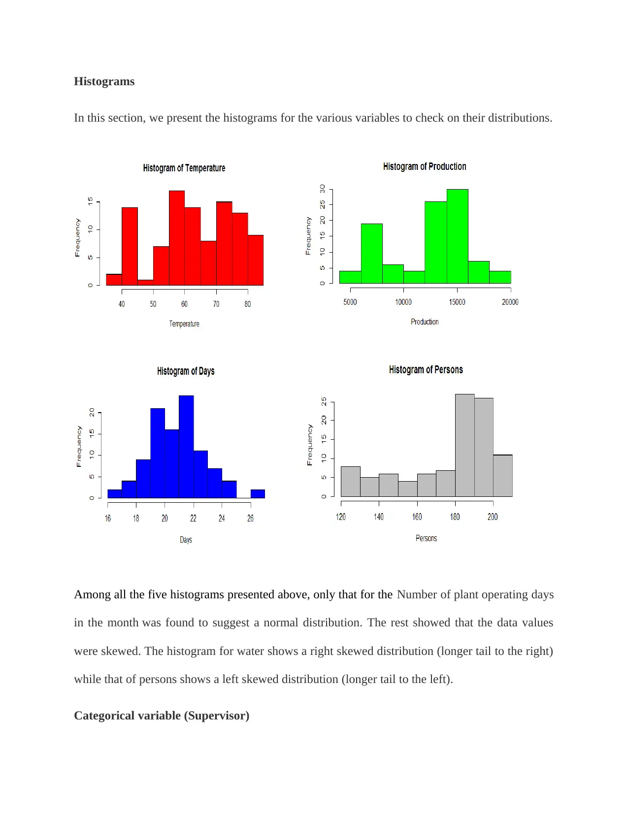
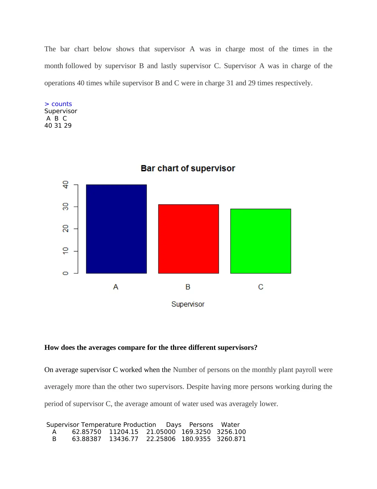
This assignment presents a comprehensive analysis of a dataset using the R programming language. The analysis begins with descriptive statistics, including measures of central tendency and dispersion, for continuous variables such as temperature, production, days, persons, and water usag...Read More

Part 1:
Descriptive Statistics
Table 1 below presents the descriptive statistics for the continuous variables. As can be seen, the
average temperature was found to be 63.33 with the highest and lowest temperatures recorded
being 82.10 and 37.70 respectively. The average production was 12332 million dollars with the
highest production cost being 18884 million dollars and lowest cost being 5574 million dollars.
Table 1: Descriptive Statistics
Temperature Production Days Persons Water
Minimum 37.70 5574 16.00 127.00 2782
1st Quarter 55.38 9119 20.00 165.50 2995
Median 64.35 13654 21.00 188.00 3085
Mean 63.33 12332 21.35 178.00 3251
3rd Quarter 72.83 14744 22.00 194.80 3486
Maximum 82.10 18884 27.00 207.00 4496
In terms of days, the average number of plant operating days in the month was 21.35 with
highest number of days being 27 and lowest number of days being 16. The average number of
persons on the monthly plant payroll was found to be 178 with the highest recorded number
being 207 while lowest recorded number being 127. Lastly, average water Monthly water usage
(gallons) was 3251 with highest usage amount being 4496 and lowest being 2782.

Histograms
In this section, we present the histograms for the various variables to check on their distributions.
Among all the five histograms presented above, only that for the Number of plant operating days
in the month was found to suggest a normal distribution. The rest showed that the data values
were skewed. The histogram for water shows a right skewed distribution (longer tail to the right)
while that of persons shows a left skewed distribution (longer tail to the left).
Categorical variable (Supervisor)

The bar chart below shows that supervisor A was in charge most of the times in the
month followed by supervisor B and lastly supervisor C. Supervisor A was in charge of the
operations 40 times while supervisor B and C were in charge 31 and 29 times respectively.
> counts
Supervisor
A B C
40 31 29
How does the averages compare for the three different supervisors?
On average supervisor C worked when the Number of persons on the monthly plant payroll were
averagely more than the other two supervisors. Despite having more persons working during the
period of supervisor C, the average amount of water used was averagely lower.
Supervisor Temperature Production Days Persons Water
A 62.85750 11204.15 21.05000 169.3250 3256.100
B 63.88387 13436.77 22.25806 180.9355 3260.871

C 63.38966 12707.34 20.79310 186.6897 3232.862
Relationship between different variables
One of the relationships we sought to investigate was the kind of relationship that exists between
temperature and water usage. The figure below presents the scatterplot between the two
variables.
As can be seen, there is a positive relationship between the temperature and the water usage. As
the temperature increase so does the water usage.

Relationship between production cost and Number of persons on the monthly plant payroll. As
can be seen, there is a positive relationship between production cost and the Number of persons
on the monthly plant payroll. This means that an increase in the Number of persons on the
monthly plant payroll would result to an increase in the production cost.

Conclusion
The results of the study showed that the average production was 12332 million dollars with the
highest production cost being 18884 million dollars and lowest cost being 5574 million dollars.
It was observed that a positive relationship exists between the temperature and the water usage;
this means that as the temperature increase so does the water usage. There is a positive
relationship between production cost and the Number of persons on the monthly plant payroll.
This means that an increase in the Number of persons on the monthly plant payroll would result
to an increase in the production cost.
Appendix
data<-read.csv("C:\\Users\\310187796\\Desktop\\waterdata.csv")
str(data)
attach(data)
library(car)
summary(data)
counts <- table(Supervisor)
counts
barplot(counts, main="Bar chart of supervisor",
xlab="Supervisor", col=c("darkblue","red", "green"))
hist(Temperature, col ="red")
hist(Production, col ="green")
hist(Days, col ="blue")
hist(Persons, col ="grey")
hist(Water, col ="purple")
aggregate(data[, 2:5], list(data$Supervisor), mean)
aggregate(data[, 7], list(data$Supervisor), mean)
plot(Temperature, Water, main="Water usage vs temperature",
xlab="Temperature", ylab="Water usage ", pch=19)
scatterplot(Production~Days, main="Production cost vs days",
xlab="Days", ylab="Production cost", pch=19)
scatterplot(Production~Persons, main="Production cost vs Persons",
xlab="Persons", ylab="Production cost", pch=19)

Output
> summary(data)
ID Temperature Production Days Persons
Min. : 1.00 Min. :37.70 Min. : 5574 Min. :16.00 Min. :127.0
1st Qu.: 52.75 1st Qu.:55.38 1st Qu.: 9119 1st Qu.:20.00 1st Qu.:165.5
Median :101.50 Median :64.35 Median :13654 Median :21.00 Median :188.0
Mean :101.98 Mean :63.33 Mean :12332 Mean :21.35 Mean :178.0
3rd Qu.:150.75 3rd Qu.:72.83 3rd Qu.:14744 3rd Qu.:22.00 3rd Qu.:194.8
Max. :199.00 Max. :82.10 Max. :18884 Max. :27.00 Max. :207.0
Supervisor Water
A:40 Min. :2782
B:31 1st Qu.:2995
C:29 Median :3085
Mean :3251
3rd Qu.:3486
Max. :4496
> counts <- table(Supervisor)
> counts
Supervisor
A B C
40 31 29
> aggregate(data[, 2:5], list(data$Supervisor), mean)
Group.1 Temperature Production Days Persons

1 A 62.85750 11204.15 21.05000 169.3250
2 B 63.88387 13436.77 22.25806 180.9355
3 C 63.38966 12707.34 20.79310 186.6897
> aggregate(data[, 7], list(data$Supervisor), mean)
Group.1 x
1 A 3256.100
2 B 3260.871
3 C 3232.862