University R Programming Assignment: Data Analysis and Bootstrapping

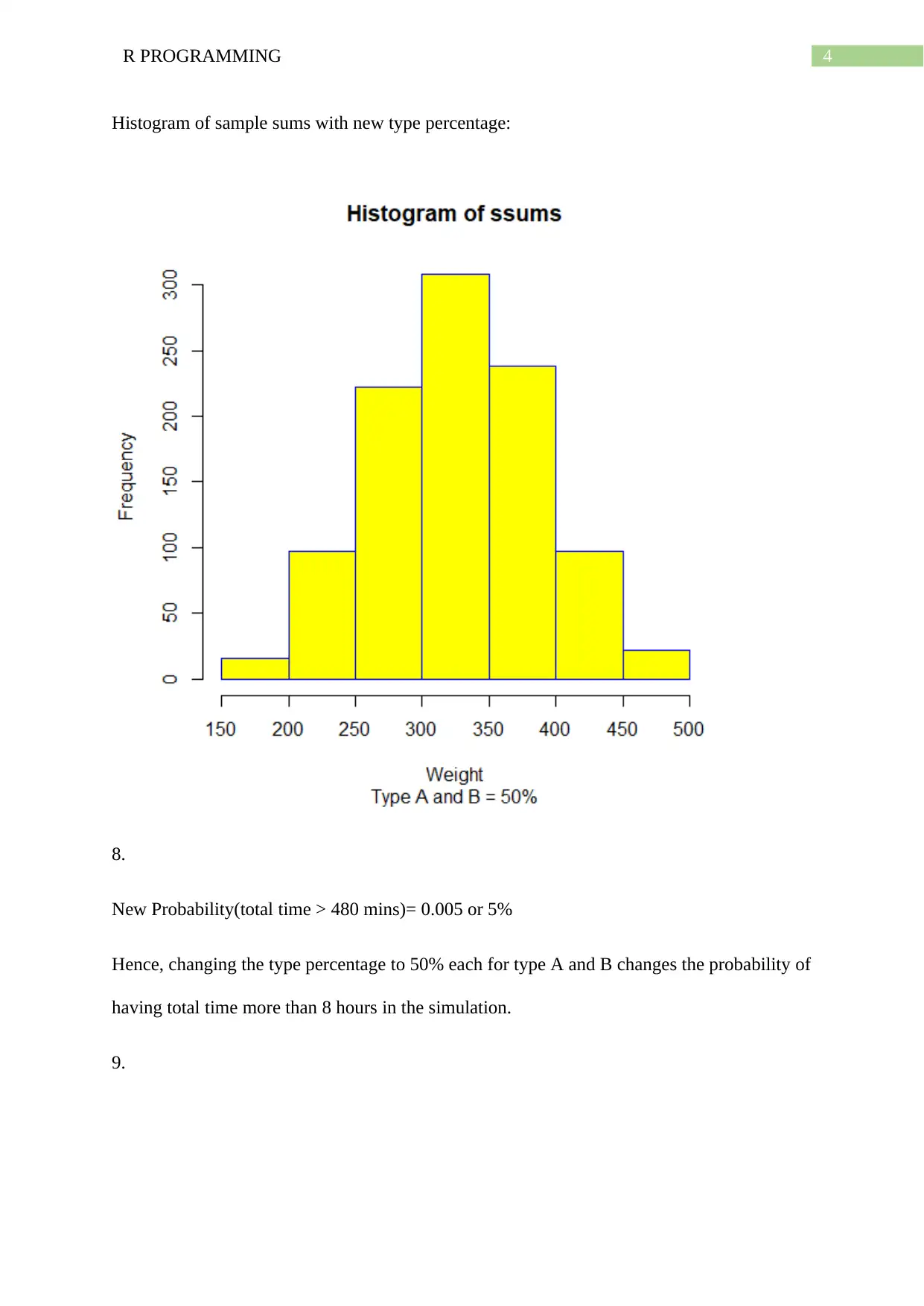
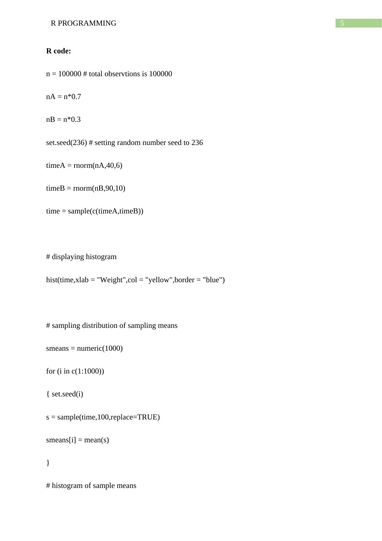
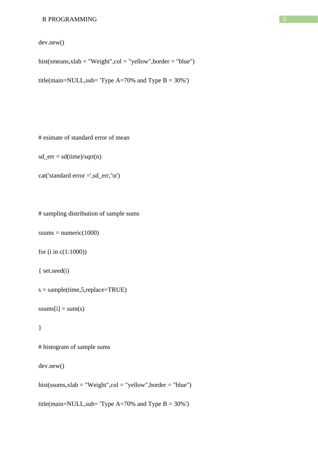
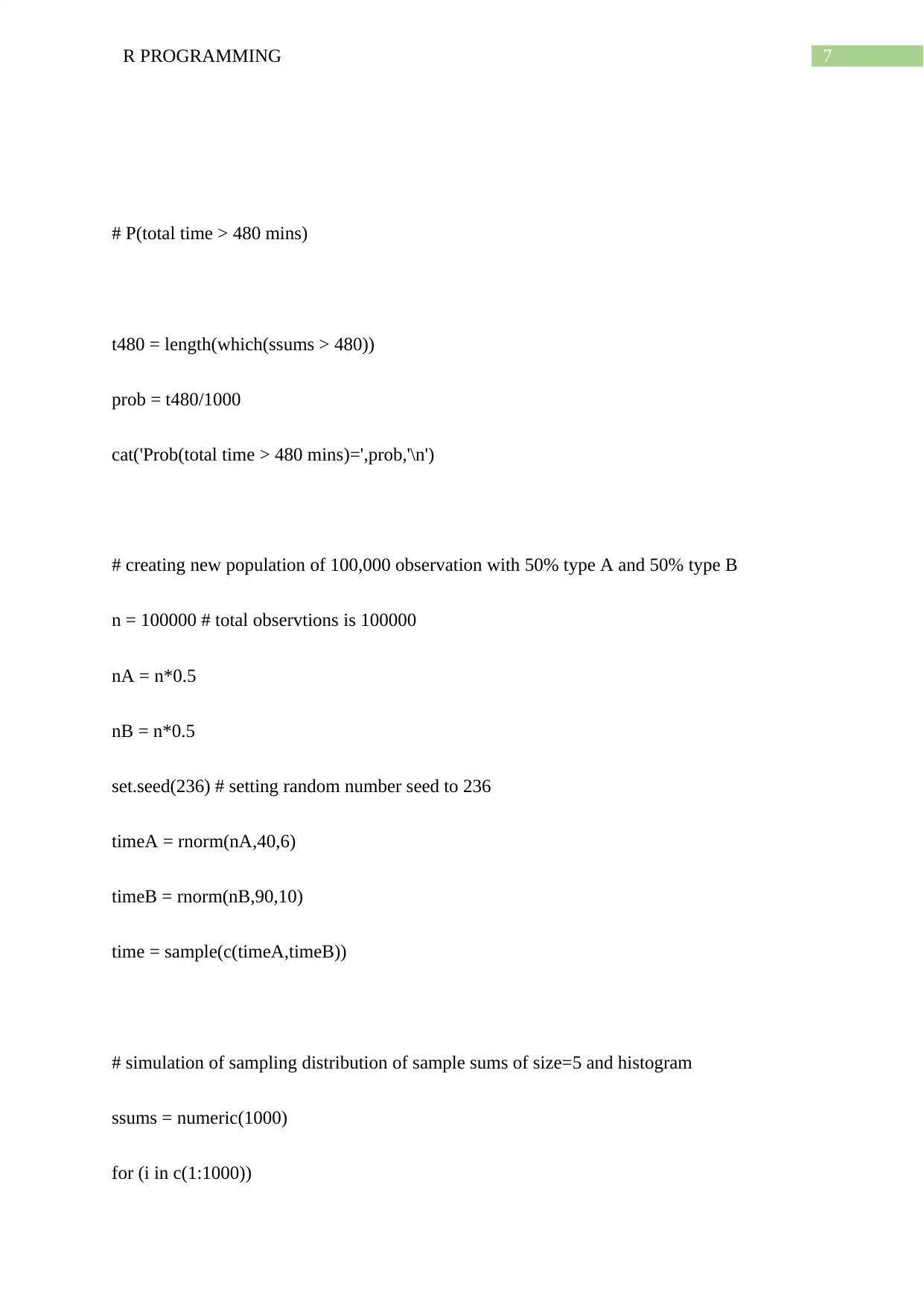
This R programming assignment focuses on data simulation and statistical analysis using the R language. Part A involves simulating a population with two types of data (A and B) following normal distributions, creating histograms, calculating standard errors, and analyzing sampling distributions of means and sums. The assignment explores how changing the type percentages impacts probabilities. Part B focuses on bootstrapping techniques to estimate confidence intervals for the Interquartile Range (IQR), comparing the standard error and percentile methods, and evaluating their accuracy. The solution includes R code for all analyses, demonstrating the practical application of statistical concepts and programming skills to analyze and interpret data, providing a comprehensive understanding of the methods used and their implications.

Running head: R PROGRAMMING
R PROGRAMMING
Name of the Student
Name of the University
Author Note

1R PROGRAMMING
Part A:
1.
Histogram of time required:
2.
Histogram of sample means:

2R PROGRAMMING
3.
Standard error =σ/sqrt(n) = 0.07620683
4.
Histogram of sample sums of 5 cases:

3R PROGRAMMING
5.
Prob(total time > 480 mins)= 0.002 or 0.2%.
6.
Now, the type percentage is changed to 50% for type A and type B and then it is simulated
for 100,000 observations with same normal distribution parameters as done in part 1.
7.

4R PROGRAMMING
Histogram of sample sums with new type percentage:
8.
New Probability(total time > 480 mins)= 0.005 or 5%
Hence, changing the type percentage to 50% each for type A and B changes the probability of
having total time more than 8 hours in the simulation.
9.

5R PROGRAMMING
R code:
n = 100000 # total observtions is 100000
nA = n*0.7
nB = n*0.3
set.seed(236) # setting random number seed to 236
timeA = rnorm(nA,40,6)
timeB = rnorm(nB,90,10)
time = sample(c(timeA,timeB))
# displaying histogram
hist(time,xlab = "Weight",col = "yellow",border = "blue")
# sampling distribution of sampling means
smeans = numeric(1000)
for (i in c(1:1000))
{ set.seed(i)
s = sample(time,100,replace=TRUE)
smeans[i] = mean(s)
}
# histogram of sample means

6R PROGRAMMING
dev.new()
hist(smeans,xlab = "Weight",col = "yellow",border = "blue")
title(main=NULL,sub= 'Type A=70% and Type B = 30%')
# esimate of standard error of mean
sd_err = sd(time)/sqrt(n)
cat('standard error =',sd_err,'\n')
# sampling distribution of sample sums
ssums = numeric(1000)
for (i in c(1:1000))
{ set.seed(i)
s = sample(time,5,replace=TRUE)
ssums[i] = sum(s)
}
# histogram of sample sums
dev.new()
hist(ssums,xlab = "Weight",col = "yellow",border = "blue")
title(main=NULL,sub= 'Type A=70% and Type B = 30%')

7R PROGRAMMING
# P(total time > 480 mins)
t480 = length(which(ssums > 480))
prob = t480/1000
cat('Prob(total time > 480 mins)=',prob,'\n')
# creating new population of 100,000 observation with 50% type A and 50% type B
n = 100000 # total observtions is 100000
nA = n*0.5
nB = n*0.5
set.seed(236) # setting random number seed to 236
timeA = rnorm(nA,40,6)
timeB = rnorm(nB,90,10)
time = sample(c(timeA,timeB))
# simulation of sampling distribution of sample sums of size=5 and histogram
ssums = numeric(1000)
for (i in c(1:1000))

8R PROGRAMMING
{ set.seed(i)
s = sample(time,5,replace=TRUE)
ssums[i] = sum(s)
}
dev.new()
hist(ssums,xlab = "Weight",col = "yellow",border = "blue")
title(main=NULL,sub= 'Type A and B = 50%')
# estimated new P(total time > 480 mins)
t480 = length(which(ssums > 480))
prob = t480/1000
cat('New Probability(total time > 480 mins)=',prob,'\n')
Part B:
1.
Bootstrapping of IQR follows these three steps
a) Sampling a specific size of data from original a large number of times.
b) Calculating IQR for each sample
c) Calculating standard deviation of the IQRs.
2.

9R PROGRAMMING
Now, by standard error method the confidence interval is found for 95% confidence by the
following formula.
CI = mean(IQR) +/- z*standard error
z = 1.96 for 95% confidence level,
standard error = σ/sqrt(n)
Now, as found using R
Lower Confidence limit = 21.51996 Higher confidence limit = 57.31996 By Standard error
method
3.
Now, quantile function is used for finding 95% confidence interval by percentile method
lower confidence corresponds to 2.5% and higher confidence corresponds to 97.5%.
Lower Confindence limit = 30 Higher confidence limit = 51 By Percentile method
4. The percentile method is more accurate than the standard error method as the accuracy of
the method depends on sample size as it can be seen from the results than confidence
intervals by two method are not same.
5.
R code:
# set working directory by function setwd() where csv file is located
datafile= read.csv(file='BerkeleyPDLog-Arrests1.csv',header=TRUE)
weight = datafile[,c(10)]
weight = weight[!is.na(weight)] # trimming missing values

10R PROGRAMMING
# bootstrapping of IQR with N=100000 and sample size n = 100
sIQR = numeric(100000)
for (i in c(1:100000))
{ set.seed(i)
s = sample(weight,100,replace=TRUE)
sIQR[i] = IQR(s)
}
# 95% confidence interval of IQR based on Standard error method
IQRmean = mean(sIQR)
z = 1.96 # for 95% confidence z value is 1.96
sigma = length(weight)
serror = sigma/sqrt(100) # standard error = sd/sqrt(n)
CIsd = c(IQRmean-serror,IQRmean+serror)
cat('Lower Confindence limit =',CIsd[1],'Higher confidence limit =',CIsd[2],'By Standard
error method')
# 95% confidence interval of IQR based on percentile method
CIpercent = quantile(sIQR,c(0.025,0.975))

11R PROGRAMMING
cat('Lower Confindence limit =',CIpercent[1],'Higher confidence limit =',CIpercent[2],'By
Percentile method')