R Programming Assignment: Data Analysis, Visualization, and Examples

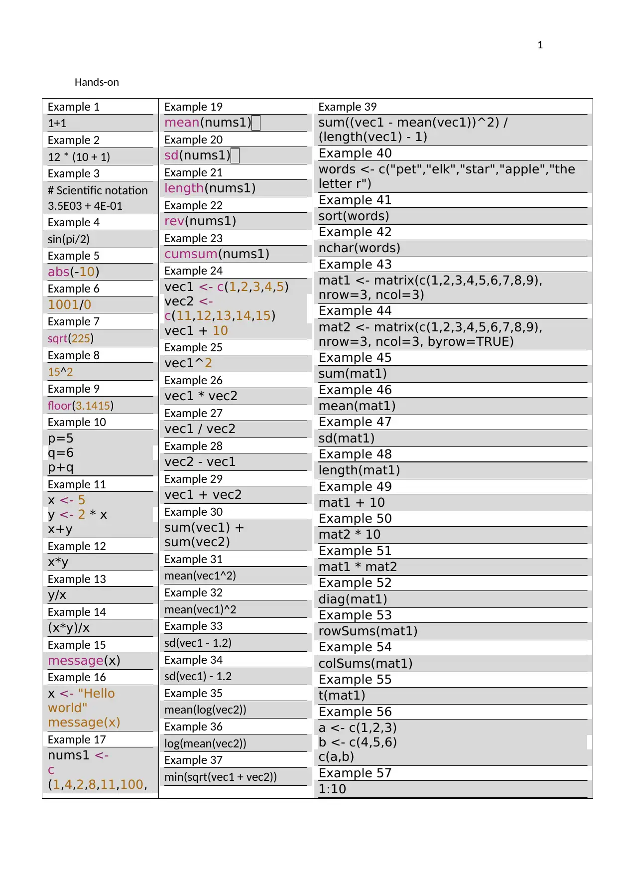
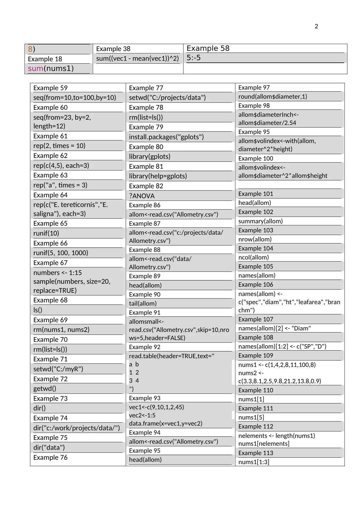
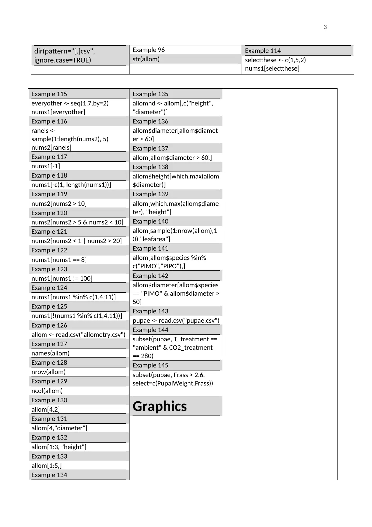
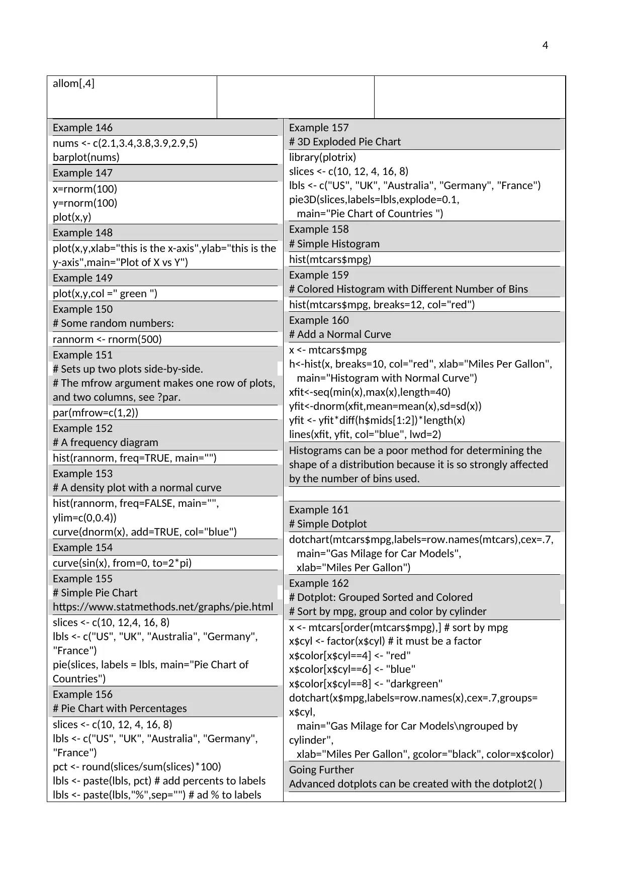
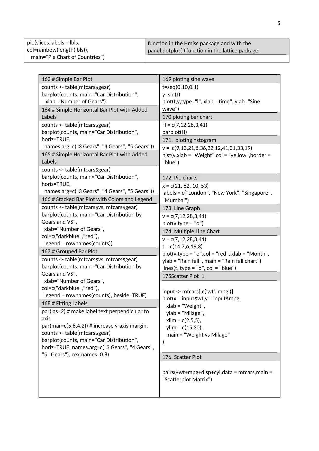
This assignment provides a comprehensive set of R programming examples, covering a wide range of data analysis and visualization techniques. The examples begin with basic operations, such as arithmetic calculations, variable assignment, and working with vectors and matrices. It progresse...Read More

1
Hands-on
Example 1
1+1
Example 2
12 * (10 + 1)
Example 3
# Scientific notation
3.5E03 + 4E-01
Example 4
sin(pi/2)
Example 5
abs(-10)
Example 6
1001/0
Example 7
sqrt(225)
Example 8
15^2
Example 9
floor(3.1415)
Example 10
p=5
q=6
p+q
Example 11
x <- 5
y <- 2 * x
x+y
Example 12
x*y
Example 13
y/x
Example 14
(x*y)/x
Example 15
message(x)
Example 16
x <- "Hello
world"
message(x)
Example 17
nums1 <-
c
(1,4,2,8,11,100,
Example 19
mean(nums1)
Example 20
sd(nums1)
Example 21
length(nums1)
Example 22
rev(nums1)
Example 23
cumsum(nums1)
Example 24
vec1 <- c(1,2,3,4,5)
vec2 <-
c(11,12,13,14,15)
vec1 + 10
Example 25
vec1^2
Example 26
vec1 * vec2
Example 27
vec1 / vec2
Example 28
vec2 - vec1
Example 29
vec1 + vec2
Example 30
sum(vec1) +
sum(vec2)
Example 31
mean(vec1^2)
Example 32
mean(vec1)^2
Example 33
sd(vec1 - 1.2)
Example 34
sd(vec1) - 1.2
Example 35
mean(log(vec2))
Example 36
log(mean(vec2))
Example 37
min(sqrt(vec1 + vec2))
Example 39
sum((vec1 - mean(vec1))^2) /
(length(vec1) - 1)
Example 40
words <- c("pet","elk","star","apple","the
letter r")
Example 41
sort(words)
Example 42
nchar(words)
Example 43
mat1 <- matrix(c(1,2,3,4,5,6,7,8,9),
nrow=3, ncol=3)
Example 44
mat2 <- matrix(c(1,2,3,4,5,6,7,8,9),
nrow=3, ncol=3, byrow=TRUE)
Example 45
sum(mat1)
Example 46
mean(mat1)
Example 47
sd(mat1)
Example 48
length(mat1)
Example 49
mat1 + 10
Example 50
mat2 * 10
Example 51
mat1 * mat2
Example 52
diag(mat1)
Example 53
rowSums(mat1)
Example 54
colSums(mat1)
Example 55
t(mat1)
Example 56
a <- c(1,2,3)
b <- c(4,5,6)
c(a,b)
Example 57
1:10

2
8)
Example 18
sum(nums1)
Example 38
sum((vec1 - mean(vec1))^2)
Example 58
5:-5
Example 59
seq(from=10,to=100,by=10)
Example 60
seq(from=23, by=2,
length=12)
Example 61
rep(2, times = 10)
Example 62
rep(c(4,5), each=3)
Example 63
rep("a", times = 3)
Example 64
rep(c("E. tereticornis","E.
saligna"), each=3)
Example 65
runif(10)
Example 66
runif(5, 100, 1000)
Example 67
numbers <- 1:15
sample(numbers, size=20,
replace=TRUE)
Example 68
ls()
Example 69
rm(nums1, nums2)
Example 70
rm(list=ls())
Example 71
setwd("C:/myR")
Example 72
getwd()
Example 73
dir()
Example 74
dir("c:/work/projects/data/")
Example 75
dir("data")
Example 76
Example 77
setwd("C:/projects/data")
Example 78
rm(list=ls())
Example 79
install.packages("gplots")
Example 80
library(gplots)
Example 81
library(help=gplots)
Example 82
?ANOVA
Example 86
allom<-read.csv("Allometry.csv")
Example 87
allom<-read.csv("c:/projects/data/
Allometry.csv")
Example 88
allom<-read.csv("data/
Allometry.csv")
Example 89
head(allom)
Example 90
tail(allom)
Example 91
allomsmall<-
read.csv("Allometry.csv",skip=10,nro
ws=5,header=FALSE)
Example 92
read.table(header=TRUE,text="
a b
1 2
3 4
")
Example 93
vec1<-c(9,10,1,2,45)
vec2<-1:5
data.frame(x=vec1,y=vec2)
Example 94
allom<-read.csv("Allometry.csv")
Example 95
head(allom)
Example 97
round(allom$diameter,1)
Example 98
allom$diameterInch<-
allom$diameter/2.54
Example 95
allom$volindex<-with(allom,
diameter^2*height)
Example 100
allom$volindex<-
allom$diameter^2*allom$height
Example 101
head(allom)
Example 102
summary(allom)
Example 103
nrow(allom)
Example 104
ncol(allom)
Example 105
names(allom)
Example 106
names(allom) <-
c("spec","diam","ht","leafarea","bran
chm")
Example 107
names(allom)[2] <- "Diam"
Example 108
names(allom)[1:2] <- c("SP","D")
Example 109
nums1 <- c(1,4,2,8,11,100,8)
nums2 <-
c(3.3,8.1,2.5,9.8,21.2,13.8,0.9)
Example 110
nums1[1]
Example 111
nums1[5]
Example 112
nelements <- length(nums1)
nums1[nelements]
Example 113
nums1[1:3]

3
dir(pattern="[.]csv",
ignore.case=TRUE)
Example 96
str(allom)
Example 114
selectthese <- c(1,5,2)
nums1[selectthese]
Example 115
everyother <- seq(1,7,by=2)
nums1[everyother]
Example 116
ranels <-
sample(1:length(nums2), 5)
nums2[ranels]
Example 117
nums1[-1]
Example 118
nums1[-c(1, length(nums1))]
Example 119
nums2[nums2 > 10]
Example 120
nums2[nums2 > 5 & nums2 < 10]
Example 121
nums2[nums2 < 1 | nums2 > 20]
Example 122
nums1[nums1 == 8]
Example 123
nums1[nums1 != 100]
Example 124
nums1[nums1 %in% c(1,4,11)]
Example 125
nums1[!(nums1 %in% c(1,4,11))]
Example 126
allom <- read.csv("allometry.csv")
Example 127
names(allom)
Example 128
nrow(allom)
Example 129
ncol(allom)
Example 130
allom[4,2]
Example 131
allom[4,"diameter"]
Example 132
allom[1:3, "height"]
Example 133
allom[1:5,]
Example 134
Example 135
allomhd <- allom[,c("height",
"diameter")]
Example 136
allom$diameter[allom$diamet
er > 60]
Example 137
allom[allom$diameter > 60,]
Example 138
allom$height[which.max(allom
$diameter)]
Example 139
allom[which.max(allom$diame
ter), "height"]
Example 140
allom[sample(1:nrow(allom),1
0),"leafarea"]
Example 141
allom[allom$species %in%
c("PIMO","PIPO"),]
Example 142
allom$diameter[allom$species
== "PIMO" & allom$diameter >
50]
Example 143
pupae <- read.csv("pupae.csv")
Example 144
subset(pupae, T_treatment ==
"ambient" & CO2_treatment
== 280)
Example 145
subset(pupae, Frass > 2.6,
select=c(PupalWeight,Frass))
Graphics

4
allom[,4]
Example 146
nums <- c(2.1,3.4,3.8,3.9,2.9,5)
barplot(nums)
Example 147
x=rnorm(100)
y=rnorm(100)
plot(x,y)
Example 148
plot(x,y,xlab="this is the x-axis",ylab="this is the
y-axis",main="Plot of X vs Y")
Example 149
plot(x,y,col =" green ")
Example 150
# Some random numbers:
rannorm <- rnorm(500)
Example 151
# Sets up two plots side-by-side.
# The mfrow argument makes one row of plots,
and two columns, see ?par.
par(mfrow=c(1,2))
Example 152
# A frequency diagram
hist(rannorm, freq=TRUE, main="")
Example 153
# A density plot with a normal curve
hist(rannorm, freq=FALSE, main="",
ylim=c(0,0.4))
curve(dnorm(x), add=TRUE, col="blue")
Example 154
curve(sin(x), from=0, to=2*pi)
Example 155
# Simple Pie Chart
https://www.statmethods.net/graphs/pie.html
slices <- c(10, 12,4, 16, 8)
lbls <- c("US", "UK", "Australia", "Germany",
"France")
pie(slices, labels = lbls, main="Pie Chart of
Countries")
Example 156
# Pie Chart with Percentages
slices <- c(10, 12, 4, 16, 8)
lbls <- c("US", "UK", "Australia", "Germany",
"France")
pct <- round(slices/sum(slices)*100)
lbls <- paste(lbls, pct) # add percents to labels
lbls <- paste(lbls,"%",sep="") # ad % to labels
Example 157
# 3D Exploded Pie Chart
library(plotrix)
slices <- c(10, 12, 4, 16, 8)
lbls <- c("US", "UK", "Australia", "Germany", "France")
pie3D(slices,labels=lbls,explode=0.1,
main="Pie Chart of Countries ")
Example 158
# Simple Histogram
hist(mtcars$mpg)
Example 159
# Colored Histogram with Different Number of Bins
hist(mtcars$mpg, breaks=12, col="red")
Example 160
# Add a Normal Curve
x <- mtcars$mpg
h<-hist(x, breaks=10, col="red", xlab="Miles Per Gallon",
main="Histogram with Normal Curve")
xfit<-seq(min(x),max(x),length=40)
yfit<-dnorm(xfit,mean=mean(x),sd=sd(x))
yfit <- yfit*diff(h$mids[1:2])*length(x)
lines(xfit, yfit, col="blue", lwd=2)
Histograms can be a poor method for determining the
shape of a distribution because it is so strongly affected
by the number of bins used.
Example 161
# Simple Dotplot
dotchart(mtcars$mpg,labels=row.names(mtcars),cex=.7,
main="Gas Milage for Car Models",
xlab="Miles Per Gallon")
Example 162
# Dotplot: Grouped Sorted and Colored
# Sort by mpg, group and color by cylinder
x <- mtcars[order(mtcars$mpg),] # sort by mpg
x$cyl <- factor(x$cyl) # it must be a factor
x$color[x$cyl==4] <- "red"
x$color[x$cyl==6] <- "blue"
x$color[x$cyl==8] <- "darkgreen"
dotchart(x$mpg,labels=row.names(x),cex=.7,groups=
x$cyl,
main="Gas Milage for Car Models\ngrouped by
cylinder",
xlab="Miles Per Gallon", gcolor="black", color=x$color)
Going Further
Advanced dotplots can be created with the dotplot2( )

5
pie(slices,labels = lbls,
col=rainbow(length(lbls)),
main="Pie Chart of Countries")
function in the Hmisc package and with the
panel.dotplot( ) function in the lattice package.
163 # Simple Bar Plot
counts <- table(mtcars$gear)
barplot(counts, main="Car Distribution",
xlab="Number of Gears")
164 # Simple Horizontal Bar Plot with Added
Labels
counts <- table(mtcars$gear)
barplot(counts, main="Car Distribution",
horiz=TRUE,
names.arg=c("3 Gears", "4 Gears", "5 Gears"))
165 # Simple Horizontal Bar Plot with Added
Labels
counts <- table(mtcars$gear)
barplot(counts, main="Car Distribution",
horiz=TRUE,
names.arg=c("3 Gears", "4 Gears", "5 Gears"))
166 # Stacked Bar Plot with Colors and Legend
counts <- table(mtcars$vs, mtcars$gear)
barplot(counts, main="Car Distribution by
Gears and VS",
xlab="Number of Gears",
col=c("darkblue","red"),
legend = rownames(counts))
167 # Grouped Bar Plot
counts <- table(mtcars$vs, mtcars$gear)
barplot(counts, main="Car Distribution by
Gears and VS",
xlab="Number of Gears",
col=c("darkblue","red"),
legend = rownames(counts), beside=TRUE)
168 # Fitting Labels
par(las=2) # make label text perpendicular to
axis
par(mar=c(5,8,4,2)) # increase y-axis margin.
counts <- table(mtcars$gear)
barplot(counts, main="Car Distribution",
horiz=TRUE, names.arg=c("3 Gears", "4 Gears",
"5 Gears"), cex.names=0.8)
169 ploting sine wave
t=seq(0,10,0.1)
y=sin(t)
plot(t,y,type="l", xlab="time", ylab="Sine
wave")
170 ploting bar chart
H = c(7,12,28,3,41)
barplot(H)
171. ploting hstogram
v = c(9,13,21,8,36,22,12,41,31,33,19)
hist(v,xlab = "Weight",col = "yellow",border =
"blue")
172. Pie charts
x = c(21, 62, 10, 53)
labels = c("London", "New York", "Singapore",
"Mumbai")
173. Line Graph
v = c(7,12,28,3,41)
plot(v,type = "o")
174. Multiple Line Chart
v = c(7,12,28,3,41)
t = c(14,7,6,19,3)
plot(v,type = "o",col = "red", xlab = "Month",
ylab = "Rain fall", main = "Rain fall chart")
lines(t, type = "o", col = "blue")
175Scatter Plot 1
input <- mtcars[,c('wt','mpg')]
plot(x = input$wt,y = input$mpg,
xlab = "Weight",
ylab = "Milage",
xlim = c(2.5,5),
ylim = c(15,30),
main = "Weight vs Milage"
)
176. Scatter Plot
pairs(~wt+mpg+disp+cyl,data = mtcars,main =
"Scatterplot Matrix")