University R Programming and Statistical Analysis Assignment
VerifiedAdded on 2023/06/03
|11
|2068
|267
Homework Assignment
AI Summary
This assignment solution demonstrates the application of R programming for statistical analysis. It begins with creating and interpreting frequency tables for categorical variables (Cylinders and Origin) from a car dataset, followed by a Chi-squared test and Cramer's V calculation to assess the association between these variables. The solution then progresses to analyzing continuous variables (MPG and Displacement), calculating descriptive statistics and performing both bivariate and multiple linear regression. The regression analyses involve setting up equations, formulating and testing hypotheses, interpreting coefficients, R-squared values, standard errors, and confidence intervals. The assignment adheres to the requirements of a social science methods course, utilizing the R programming language for data manipulation, statistical modeling, and result interpretation. The solution includes code snippets, output interpretations, and references to support the analysis.

Computer Programing Rstudio
Student name:
Student number:
Lecturer name:
31st October 2018
Student name:
Student number:
Lecturer name:
31st October 2018
Paraphrase This Document
Need a fresh take? Get an instant paraphrase of this document with our AI Paraphraser
Task 1
Online data on cars was used for this report. The link to the dataset is given below;
https://perso.telecom-paristech.fr/eagan/class/igr204/data/cars.csv
1. Create two frequency tables. Interpret and comment on the result.
Answer
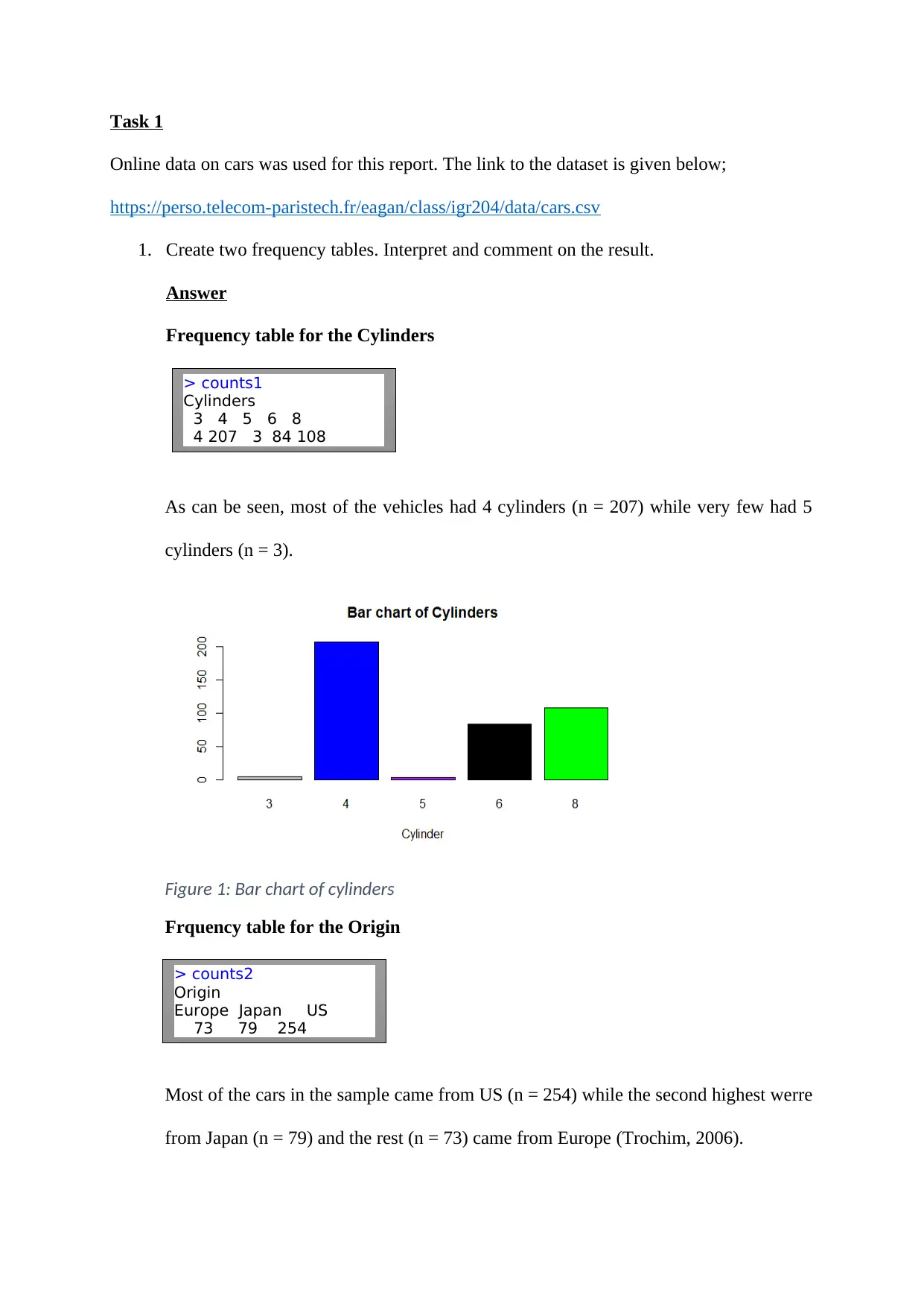
Frequency table for the Cylinders
As can be seen, most of the vehicles had 4 cylinders (n = 207) while very few had 5
cylinders (n = 3).
Figure 1: Bar chart of cylinders
Frquency table for the Origin
Most of the cars in the sample came from US (n = 254) while the second highest werre
from Japan (n = 79) and the rest (n = 73) came from Europe (Trochim, 2006).
> counts1
Cylinders
3 4 5 6 8
4 207 3 84 108
> counts2
Origin
Europe Japan US
73 79 254
Online data on cars was used for this report. The link to the dataset is given below;
https://perso.telecom-paristech.fr/eagan/class/igr204/data/cars.csv
1. Create two frequency tables. Interpret and comment on the result.
Answer
Frequency table for the Cylinders
As can be seen, most of the vehicles had 4 cylinders (n = 207) while very few had 5
cylinders (n = 3).
Figure 1: Bar chart of cylinders
Frquency table for the Origin
Most of the cars in the sample came from US (n = 254) while the second highest werre
from Japan (n = 79) and the rest (n = 73) came from Europe (Trochim, 2006).
> counts1
Cylinders
3 4 5 6 8
4 207 3 84 108
> counts2
Origin
Europe Japan US
73 79 254
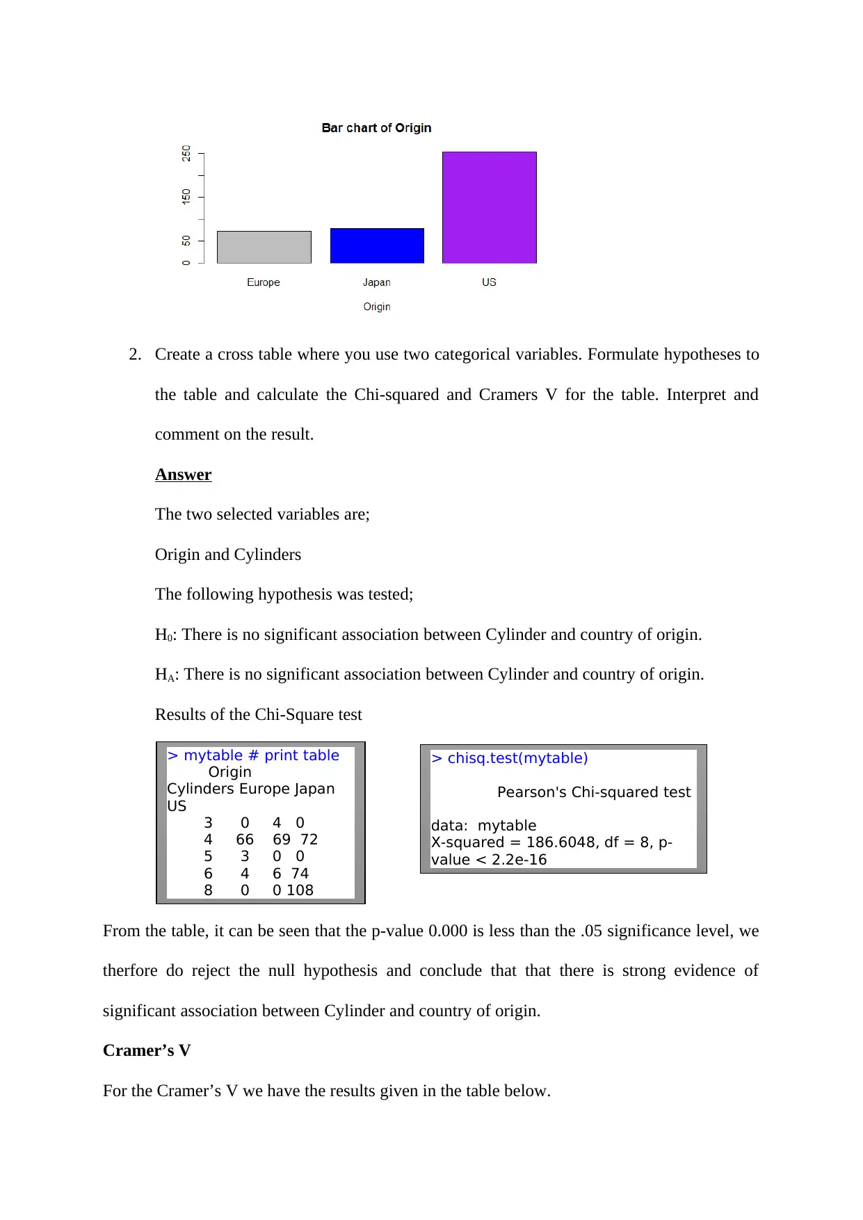
2. Create a cross table where you use two categorical variables. Formulate hypotheses to
the table and calculate the Chi-squared and Cramers V for the table. Interpret and
comment on the result.
Answer
The two selected variables are;
Origin and Cylinders
The following hypothesis was tested;
H0: There is no significant association between Cylinder and country of origin.
HA: There is no significant association between Cylinder and country of origin.
Results of the Chi-Square test
From the table, it can be seen that the p-value 0.000 is less than the .05 significance level, we
therfore do reject the null hypothesis and conclude that that there is strong evidence of
significant association between Cylinder and country of origin.
Cramer’s V
For the Cramer’s V we have the results given in the table below.
> mytable # print table
Origin
Cylinders Europe Japan
US
3 0 4 0
4 66 69 72
5 3 0 0
6 4 6 74
8 0 0 108
> chisq.test(mytable)
Pearson's Chi-squared test
data: mytable
X-squared = 186.6048, df = 8, p-
value < 2.2e-16
⊘ This is a preview!⊘
Do you want full access?
Subscribe today to unlock all pages.
Trusted by 1+ million students worldwide
Symmetric Measures
Value Approx. Sig.
Nominal by Nominal Phi .678 .000
Cramer's V .479 .000
N of Valid Cases 406
The value of Cramer’s V was found to be 0.479 which shows a moderate association between
the variables (Origin and Cylinders).
Task 2
In this task you will work with continuous and categorical variables.
You are free to choose data sets and variables yourself, either from data sets available
in Canvas or from your own source. Siter the data set you use in the task.
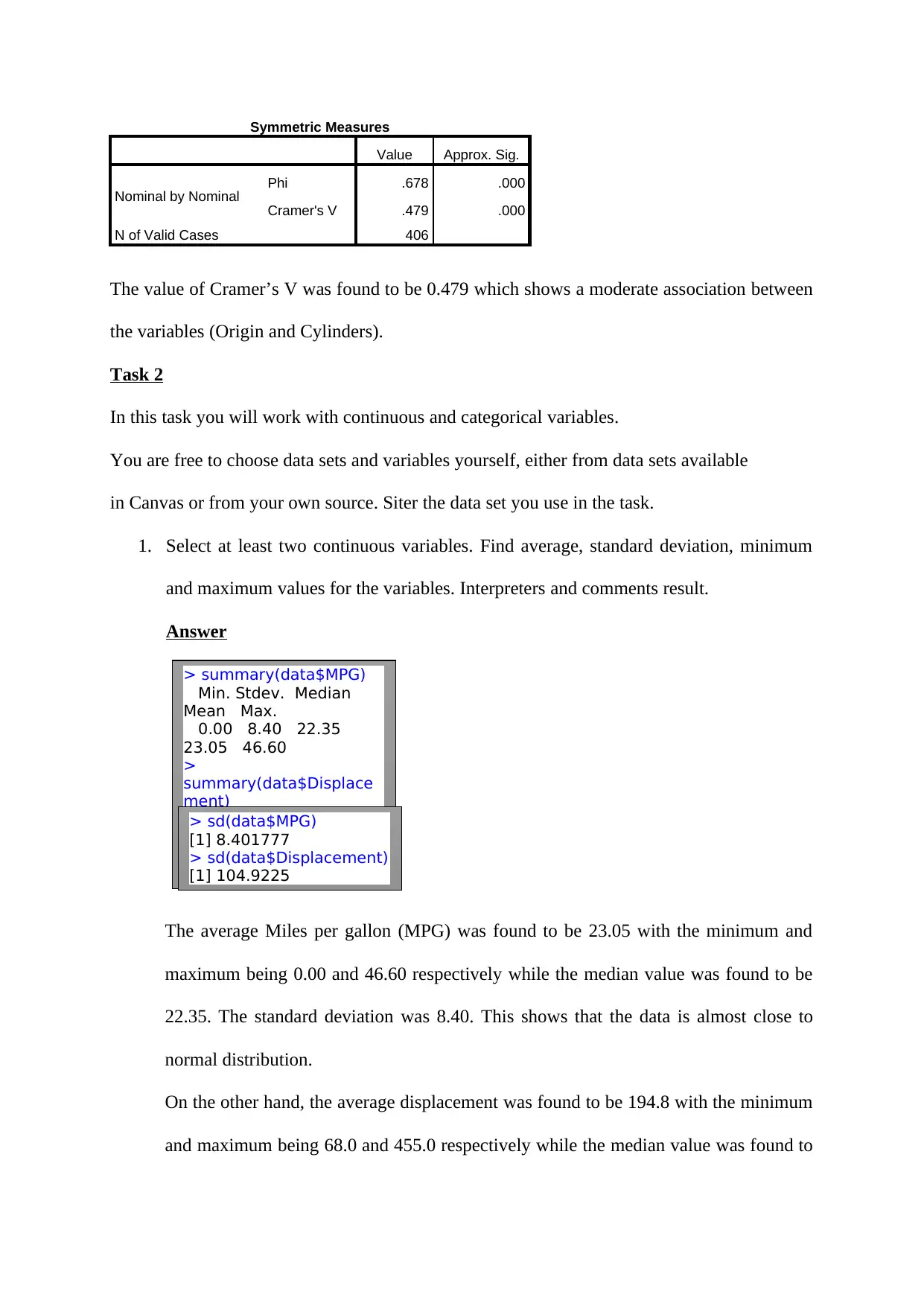
1. Select at least two continuous variables. Find average, standard deviation, minimum
and maximum values for the variables. Interpreters and comments result.
Answer
The average Miles per gallon (MPG) was found to be 23.05 with the minimum and
maximum being 0.00 and 46.60 respectively while the median value was found to be
22.35. The standard deviation was 8.40. This shows that the data is almost close to
normal distribution.
On the other hand, the average displacement was found to be 194.8 with the minimum
and maximum being 68.0 and 455.0 respectively while the median value was found to
> summary(data$MPG)
Min. Stdev. Median
Mean Max.
0.00 8.40 22.35
23.05 46.60
>
summary(data$Displace
ment)
Min. Stdev. Median
Mean Max.
68.0 104.92 151.0
194.8 455.0
> sd(data$MPG)
[1] 8.401777
> sd(data$Displacement)
[1] 104.9225
Value Approx. Sig.
Nominal by Nominal Phi .678 .000
Cramer's V .479 .000
N of Valid Cases 406
The value of Cramer’s V was found to be 0.479 which shows a moderate association between
the variables (Origin and Cylinders).
Task 2
In this task you will work with continuous and categorical variables.
You are free to choose data sets and variables yourself, either from data sets available
in Canvas or from your own source. Siter the data set you use in the task.
1. Select at least two continuous variables. Find average, standard deviation, minimum
and maximum values for the variables. Interpreters and comments result.
Answer
The average Miles per gallon (MPG) was found to be 23.05 with the minimum and
maximum being 0.00 and 46.60 respectively while the median value was found to be
22.35. The standard deviation was 8.40. This shows that the data is almost close to
normal distribution.
On the other hand, the average displacement was found to be 194.8 with the minimum
and maximum being 68.0 and 455.0 respectively while the median value was found to
> summary(data$MPG)
Min. Stdev. Median
Mean Max.
0.00 8.40 22.35
23.05 46.60
>
summary(data$Displace
ment)
Min. Stdev. Median
Mean Max.
68.0 104.92 151.0
194.8 455.0
> sd(data$MPG)
[1] 8.401777
> sd(data$Displacement)
[1] 104.9225
Paraphrase This Document
Need a fresh take? Get an instant paraphrase of this document with our AI Paraphraser
be 151.0. The standard deviation was 104.94. This shows that the data is almost close
to normal distribution since there is no uch spread in the data.
2. Perform a bivariate linear regression analysis with two continuous variables.
You shall: Set up the equation, interpret and comment on the result.
Formulate hypotheses for the variables. Conclude the hypothesis. Interpret the
explained variance (R-squared). Comment on default errors and contexts.
Answer
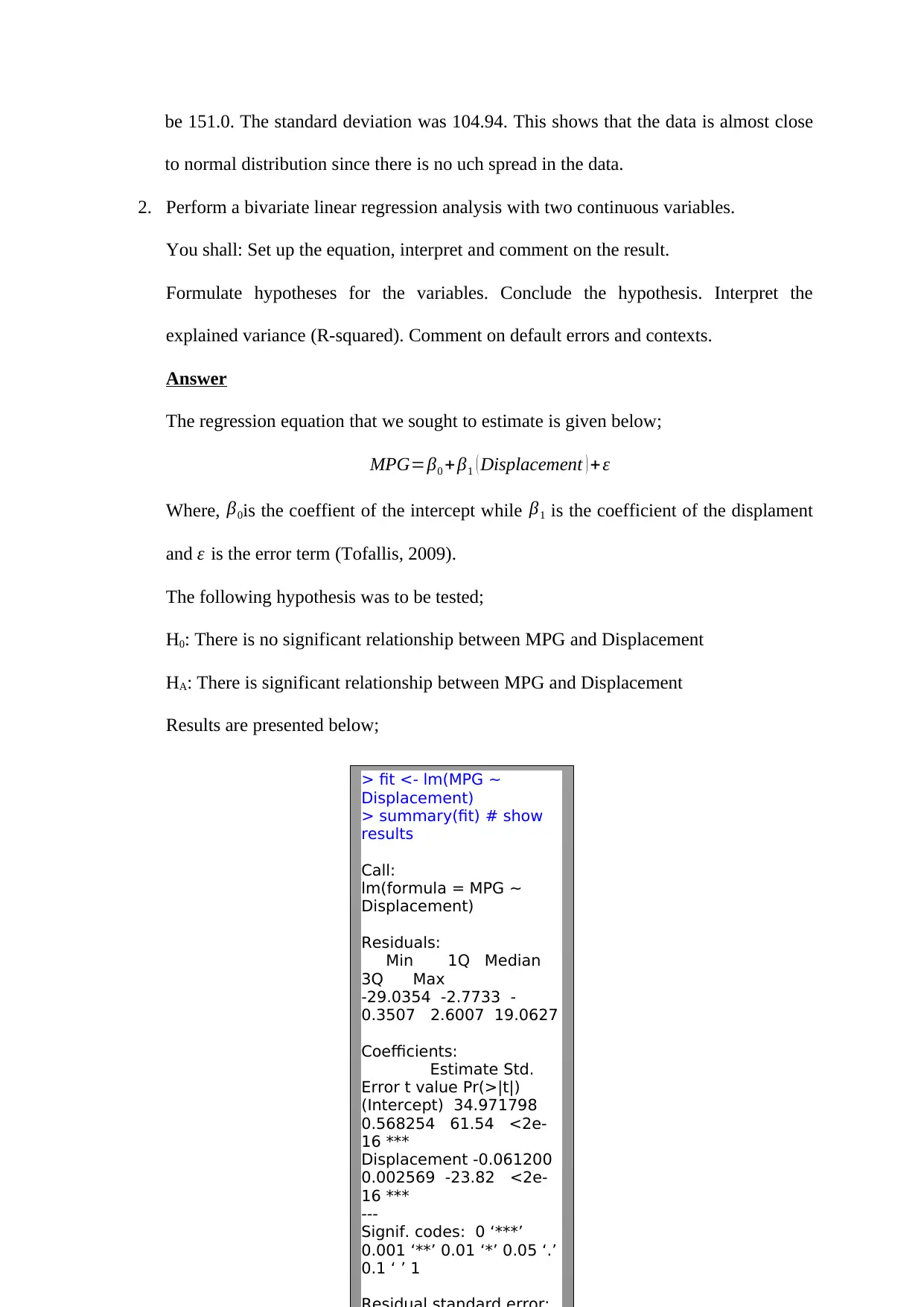
The regression equation that we sought to estimate is given below;
MPG=β0 +β1 ( Displacement ) +ε
Where, β0is the coeffient of the intercept while β1 is the coefficient of the displament
and ε is the error term (Tofallis, 2009).
The following hypothesis was to be tested;
H0: There is no significant relationship between MPG and Displacement
HA: There is significant relationship between MPG and Displacement
Results are presented below;
> fit <- lm(MPG ~
Displacement)
> summary(fit) # show
results
Call:
lm(formula = MPG ~
Displacement)
Residuals:
Min 1Q Median
3Q Max
-29.0354 -2.7733 -
0.3507 2.6007 19.0627
Coefficients:
Estimate Std.
Error t value Pr(>|t|)
(Intercept) 34.971798
0.568254 61.54 <2e-
16 ***
Displacement -0.061200
0.002569 -23.82 <2e-
16 ***
---
Signif. codes: 0 ‘***’
0.001 ‘**’ 0.01 ‘*’ 0.05 ‘.’
0.1 ‘ ’ 1
to normal distribution since there is no uch spread in the data.
2. Perform a bivariate linear regression analysis with two continuous variables.
You shall: Set up the equation, interpret and comment on the result.
Formulate hypotheses for the variables. Conclude the hypothesis. Interpret the
explained variance (R-squared). Comment on default errors and contexts.
Answer
The regression equation that we sought to estimate is given below;
MPG=β0 +β1 ( Displacement ) +ε
Where, β0is the coeffient of the intercept while β1 is the coefficient of the displament
and ε is the error term (Tofallis, 2009).
The following hypothesis was to be tested;
H0: There is no significant relationship between MPG and Displacement
HA: There is significant relationship between MPG and Displacement
Results are presented below;
> fit <- lm(MPG ~
Displacement)
> summary(fit) # show
results
Call:
lm(formula = MPG ~
Displacement)
Residuals:
Min 1Q Median
3Q Max
-29.0354 -2.7733 -
0.3507 2.6007 19.0627
Coefficients:
Estimate Std.
Error t value Pr(>|t|)
(Intercept) 34.971798
0.568254 61.54 <2e-
16 ***
Displacement -0.061200
0.002569 -23.82 <2e-
16 ***
---
Signif. codes: 0 ‘***’
0.001 ‘**’ 0.01 ‘*’ 0.05 ‘.’
0.1 ‘ ’ 1
The p-value was for the displacement was found to be 0.000 (a value less than 5%
level of significance), we therefore reject the null hypothesis and conclude that there is
significant relationship between MPG and Displacement. The coefficient for
displacement was found to be -0.0612; this suggests that a unit increase in
displacement would result in reduction in the MPG by 0.0612.
The R-squared value is given as 0.5841; this means that 58.41% of the variation in the
miles per gallon (MPG) is explained by the displacement (explanatory variable) in the
model. Close to 41% of the variation in MPG is explained by the error term (variables
outside the model).
The final regression model is thus;
MPG=34.9718−0.0612 ( Displacement )
The standard error for the explanatory variable (displacement) is iven as 0.0026;
which tells us that the average distance of the data points from the fitted line is about
0..0026 displacement.
3. Perform a multiple linear regression analysis with at least three independent variables.
You shall: Set up the equation, interpret and comment on the result. Formulate
hypotheses for two of the variables in the model. concluding hypotheses. Interpret the
explained variance (R-squared). Comment on standard errors and Confidence interval.
Answer
The regression equation that we sought to estimate is given below;
MPG=β0 + β1 ( Displacement ) + β2 ( Weight ) + β3 ( Acceleration ) +ε
Where, β0is the coeffient of the intercept while β1 is the coefficient for the displament,
β2 is the coefficient for the weight, β3 is the coefficient for the acceleration and ε is the
error term (Fisher, 2002).
The following hypothesis were to be tested;
⊘ This is a preview!⊘
Do you want full access?
Subscribe today to unlock all pages.
Trusted by 1+ million students worldwide
i) H0: There is no significant relationship between MPG and Displacement
HA: There is significant relationship between MPG and Displacement
ii) H0: There is no significant relationship between MPG and Weight
HA: There is significant relationship between MPG and Weight
iii) H0: There is no significant relationship between MPG and Acceleration
HA: There is significant relationship between MPG and Acceleration
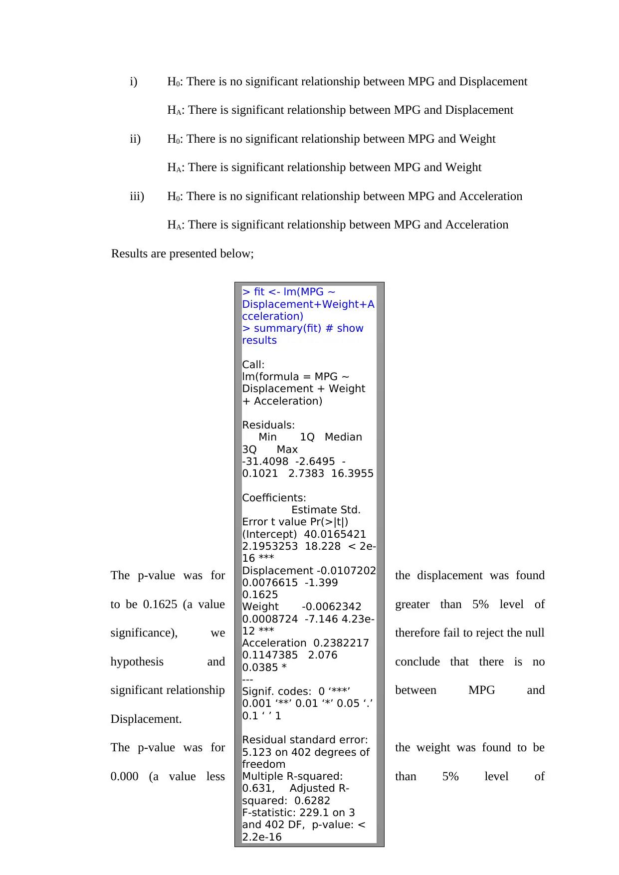
Results are presented below;
The p-value was for the displacement was found
to be 0.1625 (a value greater than 5% level of
significance), we therefore fail to reject the null
hypothesis and conclude that there is no
significant relationship between MPG and
Displacement.
The p-value was for the weight was found to be
0.000 (a value less than 5% level of
> fit <- lm(MPG ~
Displacement+Weight+A
cceleration)
> summary(fit) # show
results
Call:
lm(formula = MPG ~
Displacement + Weight
+ Acceleration)
Residuals:
Min 1Q Median
3Q Max
-31.4098 -2.6495 -
0.1021 2.7383 16.3955
Coefficients:
Estimate Std.
Error t value Pr(>|t|)
(Intercept) 40.0165421
2.1953253 18.228 < 2e-
16 ***
Displacement -0.0107202
0.0076615 -1.399
0.1625
Weight -0.0062342
0.0008724 -7.146 4.23e-
12 ***
Acceleration 0.2382217
0.1147385 2.076
0.0385 *
---
Signif. codes: 0 ‘***’
0.001 ‘**’ 0.01 ‘*’ 0.05 ‘.’
0.1 ‘ ’ 1
Residual standard error:
5.123 on 402 degrees of
freedom
Multiple R-squared:
0.631, Adjusted R-
squared: 0.6282
F-statistic: 229.1 on 3
and 402 DF, p-value: <
2.2e-16
HA: There is significant relationship between MPG and Displacement
ii) H0: There is no significant relationship between MPG and Weight
HA: There is significant relationship between MPG and Weight
iii) H0: There is no significant relationship between MPG and Acceleration
HA: There is significant relationship between MPG and Acceleration
Results are presented below;
The p-value was for the displacement was found
to be 0.1625 (a value greater than 5% level of
significance), we therefore fail to reject the null
hypothesis and conclude that there is no
significant relationship between MPG and
Displacement.
The p-value was for the weight was found to be
0.000 (a value less than 5% level of
> fit <- lm(MPG ~
Displacement+Weight+A
cceleration)
> summary(fit) # show
results
Call:
lm(formula = MPG ~
Displacement + Weight
+ Acceleration)
Residuals:
Min 1Q Median
3Q Max
-31.4098 -2.6495 -
0.1021 2.7383 16.3955
Coefficients:
Estimate Std.
Error t value Pr(>|t|)
(Intercept) 40.0165421
2.1953253 18.228 < 2e-
16 ***
Displacement -0.0107202
0.0076615 -1.399
0.1625
Weight -0.0062342
0.0008724 -7.146 4.23e-
12 ***
Acceleration 0.2382217
0.1147385 2.076
0.0385 *
---
Signif. codes: 0 ‘***’
0.001 ‘**’ 0.01 ‘*’ 0.05 ‘.’
0.1 ‘ ’ 1
Residual standard error:
5.123 on 402 degrees of
freedom
Multiple R-squared:
0.631, Adjusted R-
squared: 0.6282
F-statistic: 229.1 on 3
and 402 DF, p-value: <
2.2e-16
Paraphrase This Document
Need a fresh take? Get an instant paraphrase of this document with our AI Paraphraser
significance), we therefore reject the null hypothesis and conclude that there is
significant relationship between MPG and Weight.
The p-value was for the Acceleration was found to be 0.0385 (a value less than 5%
level of significance), we therefore reject the null hypothesis and conclude that there is
significant relationship between MPG and Acceleration.
The R-squared value is given as 0.631; this means that 63.1% of the variation in the
miles per gallon (MPG) is explained by the three explanatory variables in the model
(displacement, weight and acceleration).
The final regression model is thus;
MPG=40.0165−0.0107 ( Displacement ) −0.0062 ( Weight ) +0.2388( Acceleration)
The standard error for the explanatory variable (displacement) is iven as 0.0077;
which tells us that the average distance of the data points from the fitted line is about
0..0077 displacement.
The standard error for the explanatory variable (weight) is iven as 0.0009; which tells
us that the average distance of the data points from the fitted line is about 0..0009
weight.
The standard error for the explanatory variable (acceleration) is iven as 0.1147; which
tells us that the average distance of the data points from the fitted line is about 0..1147
acceleration.
The confidence interval for the explaanatory variables also shows that two of the three
expalantory variables are significant.
References
Fisher, R. A. (2002). The goodness of fit of regression formulae, and the distribution of
regression coefficients. Journal of the Royal Statistical Society, 85(4), 597–612.
Tofallis, C. (2009). Least Squares Percentage Regression. Journal of Modern Applied
Statistical Methods, 7, 526–534.
Trochim, W. M. (2006). Descriptive statistics. Research Methods Knowledge Base.
⊘ This is a preview!⊘
Do you want full access?
Subscribe today to unlock all pages.
Trusted by 1+ million students worldwide

Appendix
data<-read.csv("C:\\Users\\310187796\\Desktop\\cars.csv")
attach(data)
str(data)
#Frequency table for Cylinders
counts1 <- table(Cylinders)
barplot(counts1, main="Bar chart of Cylinders",
xlab="Cylinder", col=c("grey","blue", "purple", "black", "green"))
counts1
#Frequency table fro the Origin
counts2 <- table(Origin)
Paraphrase This Document
Need a fresh take? Get an instant paraphrase of this document with our AI Paraphraser
barplot(counts2, main="Bar chart of Origin",
xlab="Origin", col=c("grey","blue", "purple"))
counts2
#Chi-Sqaure table
mytable <- table(Cylinders,Origin) # A will be rows, B will be columns
mytable # print table
chisq.test(mytable)
#Summary statistics
summary(data$MPG)
summary(data$Displacement)
sd(data$MPG)
sd(data$Displacement)
#Simple Regression analysis
fit <- lm(MPG ~ Displacement)
summary(fit) # show results
#Multiple Regression analysis
fit <- lm(MPG ~ Displacement+Weight+Acceleration)
summary(fit) # show results
1 out of 11
Your All-in-One AI-Powered Toolkit for Academic Success.
+13062052269
info@desklib.com
Available 24*7 on WhatsApp / Email
![[object Object]](/_next/static/media/star-bottom.7253800d.svg)
Unlock your academic potential
Copyright © 2020–2026 A2Z Services. All Rights Reserved. Developed and managed by ZUCOL.